Estimate Powerlaw

The power law relationship that we are interested in studying within this work is one between mean rankand parcellation size. A key trait of powerlaw distributions, especially those noted within this work, are that they only exist or are observed within a certain range. That is to say, their exists a region of parcellation sizes in which a relationship might hold, but this will not extend infinitely. For example let’s consider the figure from Intro to Results which shows the log10-log10 results from the Elastic-Net and randomly generated parcellations. A line of best fit is included according to an ordinary least squares (OLS) regression, formula log10(Mean Rank) ~ log10(Size).

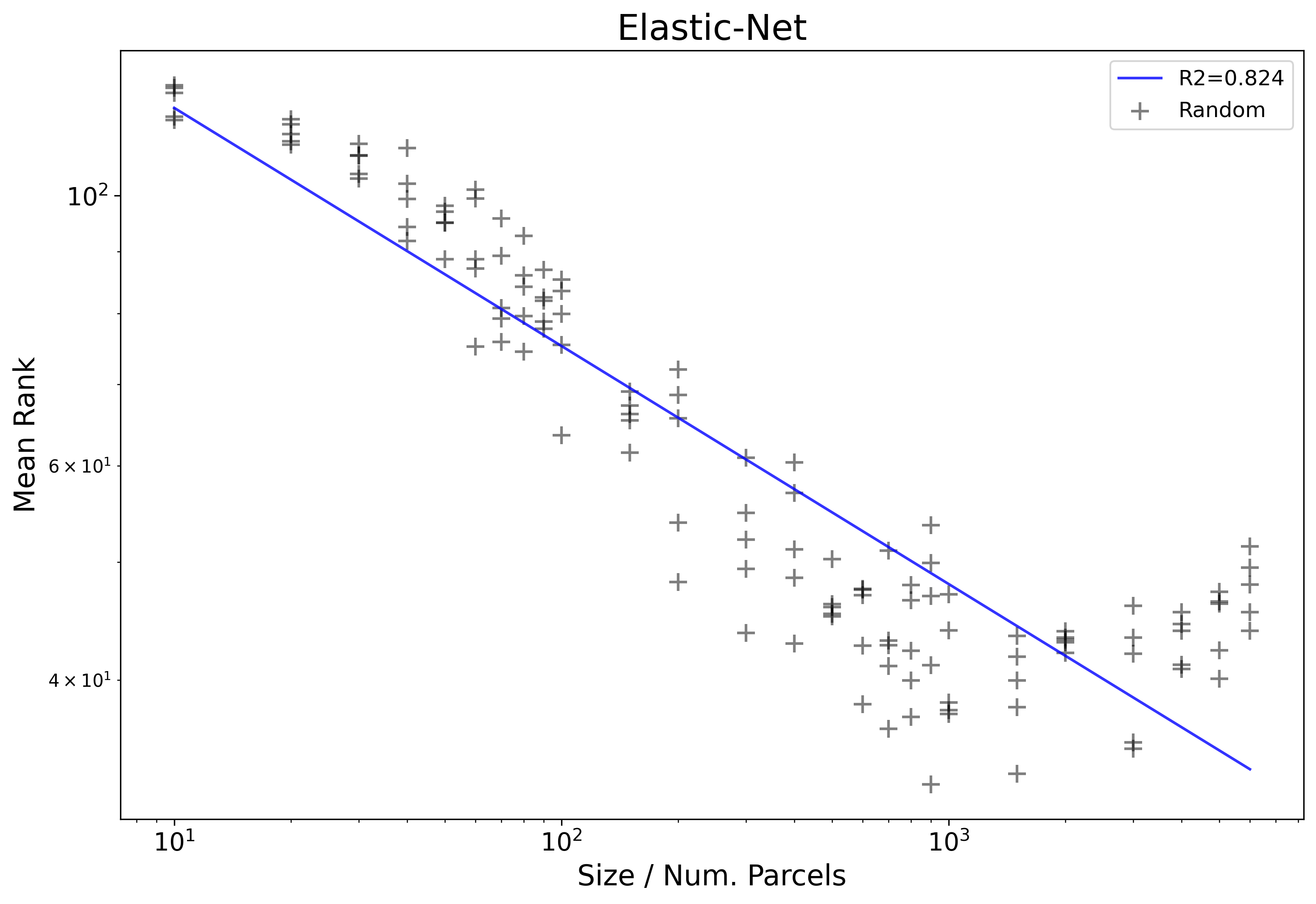
The first thing that stands out from this figure just visually is that the initial linear pattern continues until about 10^3 and then plateaus, followed by spiking upward. The idea here is that the spike at the end represents sizes where the powerlaw distribution fails to hold, and therefore those results start to mess up the clean linear relationship visible in the smaller sizes (and also the OLS fit at R2=.824). We can also not visually that because of the jump at the end, the plotted line doesn’t follow the observed results very well.

What if we could instead just the model the results up to about size 10^3? The problem here is how do we decide on that number, as just sort of eye-balling the log10-log10 plot is not exactly rigorous and reproducible. Instead, we must first introduce an automated way of estimating the region where the powerlaw relationship holds. We will use a method based off this paper by Aaron Clauset, with some slight adjustments. The fundamental idea is we will be comparing how well different samples of the observed data fits to the expected powerlaw distribution.

• As a first pass, we start by determining the lower threshold, that is to say, the cut-off where sizes below a threshold should not be included. We then apply this threshold and next calculate the upper threshold in the same manner. The order here was decided arbitrarily, but hopefully should not influence the results too much.

• We then check the KS Statistic between the real data and the expected distribution, specifically:

    from scipy.stats import linregress, kstest
    import numpy as np
    
    # xs are the sizes and ys are the mean ranks
    # we first fit a linear regression on the log10 of each
    r = linregress(np.log10(xs), np.log10(ys))
    
    # We can then compute the predicted points under the assumption
    # that these real data points perfectly fit a powerlaw distribution
    p_ys = 10**(r.intercept) * (xs **(r.slope))
    
    # Lastly, we compute the KS statistic between the real and expected fit
    k = kstest(ys, p_ys).statistic

• We compute the KS Statistic first for all data points, then all but the smallest, then all but the second smallest and so on up until at most the smallest 1/4 are removed. The threshold, in this case the lower threshold, is then determined by selecting the subset of data which minimizes the KS statistic. When computing the upper threshold the same procedure is repeated except with the largest data points and with the lower threshold already applied.

Returning to the example from earlier, if we run the described procedure, we can then plot just the OLS fit from between the two automatically computed thresholds:

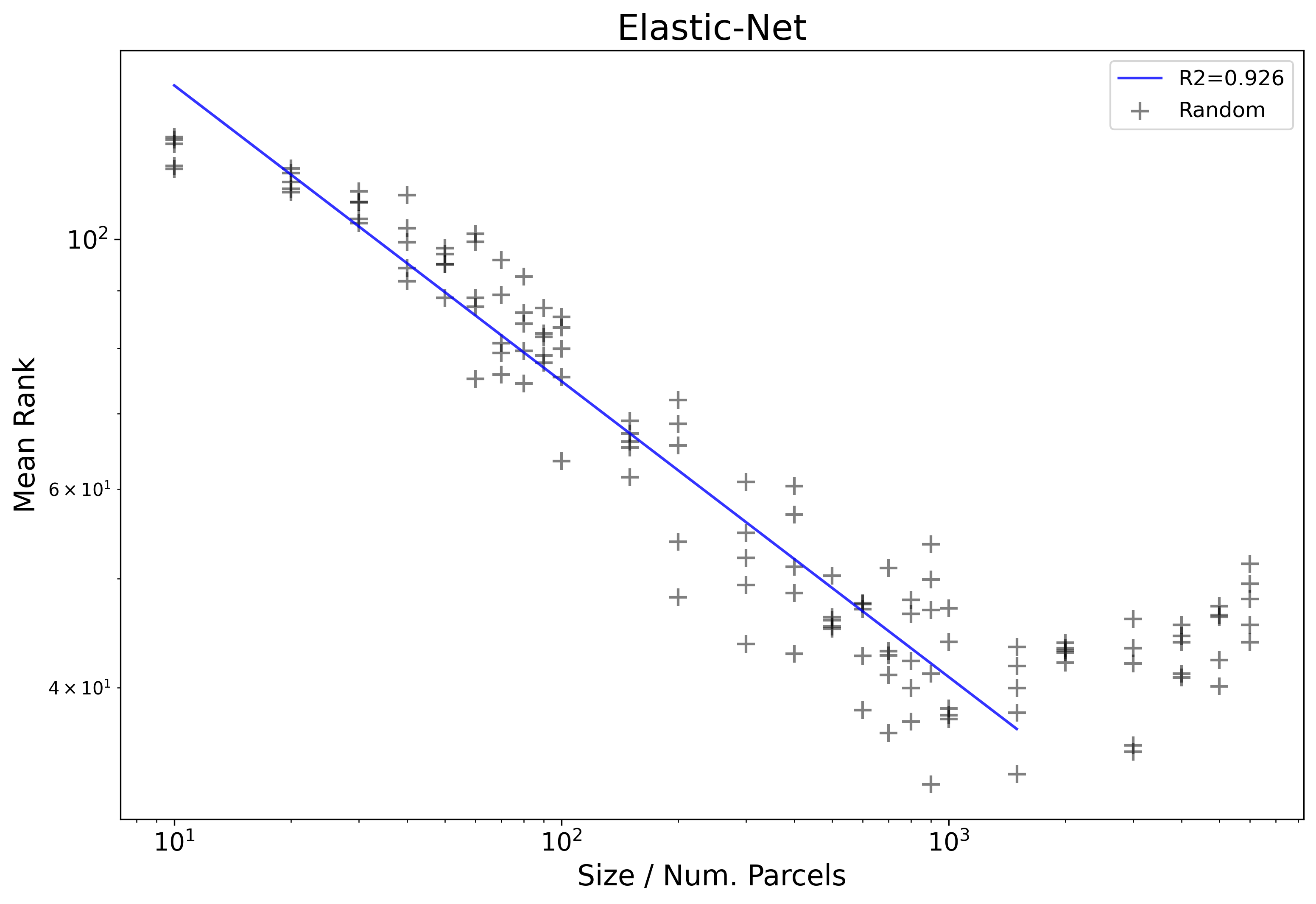
We can now see that the line matches much closer to the data-points (R2=.926) as well as matches roughly to the visually / intuitively defined threshold. Correctly identifying this region is important because it greatly influences the estimated slope or exponent of power-law scaling, and also practically it helps to identify where performance actually gets worse when adding more parcels.

Code

The whole relevant code is contained in the functions below:

    def get_divergence(ij, in_xs, in_ys, plot=False):
        
        i, j = ij
        
        if i < 0 or j < 0:
            return 10000
        
        j = -j
        if j == 0:
            j = None
        
        xs = in_xs.copy()[i:j]
        ys = in_ys.copy()[i:j]
        
        # Estimate fit
        r = linregress(np.log10(xs), np.log10(ys))
        
        # Get points from what should be fit
        p_ys = 10**(r.intercept) * (xs **(r.slope))
        
        k = kstest(ys, p_ys).statistic
        
        if plot:
            plt.scatter(xs, p_ys)
            plt.scatter(xs, ys)
        
        # Return kstest
        return k

    def get_min_max_bounds(r_df, plot=False):
        
        # To array
        xs = np.array(r_df['Size'])
        ys = np.array(r_df['Mean_Rank'])
    
        up_to = len(xs) // 4

        # First estimate lower bound
        options = [(i, 0) for i in range(up_to)]
        divergences = [get_divergence(o, xs, ys) for o in options]
        i = options[np.argmin(divergences)][0]

        # Estimate upper based on lower
        options = [(i, j) for j in range(up_to)]
        divergences = [get_divergence(o, xs, ys) for o in options]
        j = options[np.argmin(divergences)][1]
        
        if plot:
            get_divergence((i, j), xs, ys, plot=True)
            
        return i, j