Intro to Results

This page includes some introductory information on some key ingredients for making sense of the results within the project.

Mean Rank

The measure of performance presented within with project is typically in terms of ‘Mean Rank’. This measure can be potentially confusing as it can change subtly from figure to figure. In the most simple case though, Mean Rank, is as the name suggests, just an average of a parcellations ‘ranks’, where a parcellations rank is generated by comparing its performance to other parcellations (when evaluated with the same ML Pipeline and for the same target variable). For example consider the highly simplified example below:

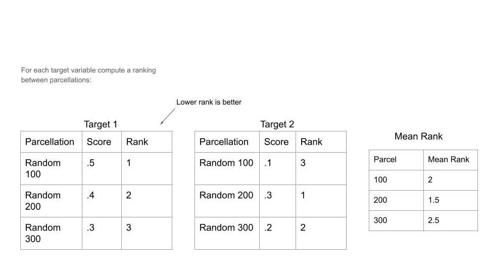
In this case, rankings are computed across three different parcellations, each which have just a generic “score” (which in the rest of the project depends on if the target variable is binary or regression, but in both cases higher is better). Then rankings are assigned individually for each of two target variables, here just Target 1 and 2, where the parcellation with the highest score gets Rank 1, then the parcellation with the next highest score gets rank 2 and so on. Mean Rank can then be computed across in this case the separate ranks for each of the two target variables. Or for example, Mean Rank could be computed both across different Target Variables and / or across different ML Pipelines, depending on the specific figure or subset of results.

A key benefit of Mean Rank over employing metrics like R2 directly is that we can now compare across both different binary and regression metrics, as well as to address scaling issues between metrics (e.g., Sex at Birth is more predictive than KSADS ADHD Composite).

In some degenerative cases Mean Rank has the potential to hide information about magnitude of difference, but in general when computed over a sufficient number of comparisons (in this case different parcellations) then this will be less of an issue. For example consider that if two parcellations varied only by a very slight amount in performance, then their mean rank as computed across many target variables would end up being very close, as each each evaluated target will be noisy. On the other hand, if a parcellation outperforms another by a large amount across a large number of target variables, then this will be accurately reflected as the better parcellation obtaining a much better Mean Rank. The core idea here is that if the difference in performance is too small between two parcellations, i.e., not actually better, then Mean Rank when computed across enough individual rankings will correctly show the two parcellations to have equivalent rank.

That said, while the magnitude of differences in performance is partially preserved by using R2 and ROC AUC directly, this information becomes muddled if not fully corrupted when averaging across multiple target variables. The reason why this occurs is the same as discussed earlier with respect to the different scaling of predictability for different target variables. We would even go so far as to argue that any remaining information of the magnitude of differences left after averaging across multiple targets is potentially misleading, not just less informative. This point is also directly related to the notion that the results when presented as mean rank have lost their immediate connection to a standard reference, whereas the averaged R2 and ROC AUC results have not. We note that when averaging across 22 or 23 variables, mean R2 or mean ROC AUC also loses its intuitive reference.

Alternative Ranks

Instead of Mean Rank, we could also instead just use the median when averaging across multiple target variables. This Median rank may provide an interesting alternative way of summarizing across 45 targets (where a simple mean would still be used when necessary to average across the three pipelines). We could also likewise perform comparisons instead with either the Maximum or Minimum rank. These would correspond interestingly in the case of Max Rank to the worst case performance of a parcellation and in the case of Min Rank, the best case performance for a parcellation.

Modelling Results

We employ ordinary least squares regression (OLS), as implemented in the python package statsmodels to model results from the base experiments. Base notation for OLS equations are written in the R formula style as A ~ B + C where A is the dependent variable and B + C are independent fixed effects. Alternatively, if written as A ~ B * D then D will be added as a fixed effect along with an interaction term between B and D (equivalent to alternate notation A ~ B + D + B * D). If a fixed effect is categorical, then it is dummy coded and each dummy variable added as a fixed effect. A variable is specified as categorical in statsmodel by wrapping it with C, for example: C(variable), would specify that variable as categorical. Lastly, if a variable is wrapped in log10(), then the logarithm of the variable with base 10 has been used.

Elastic-Net Example

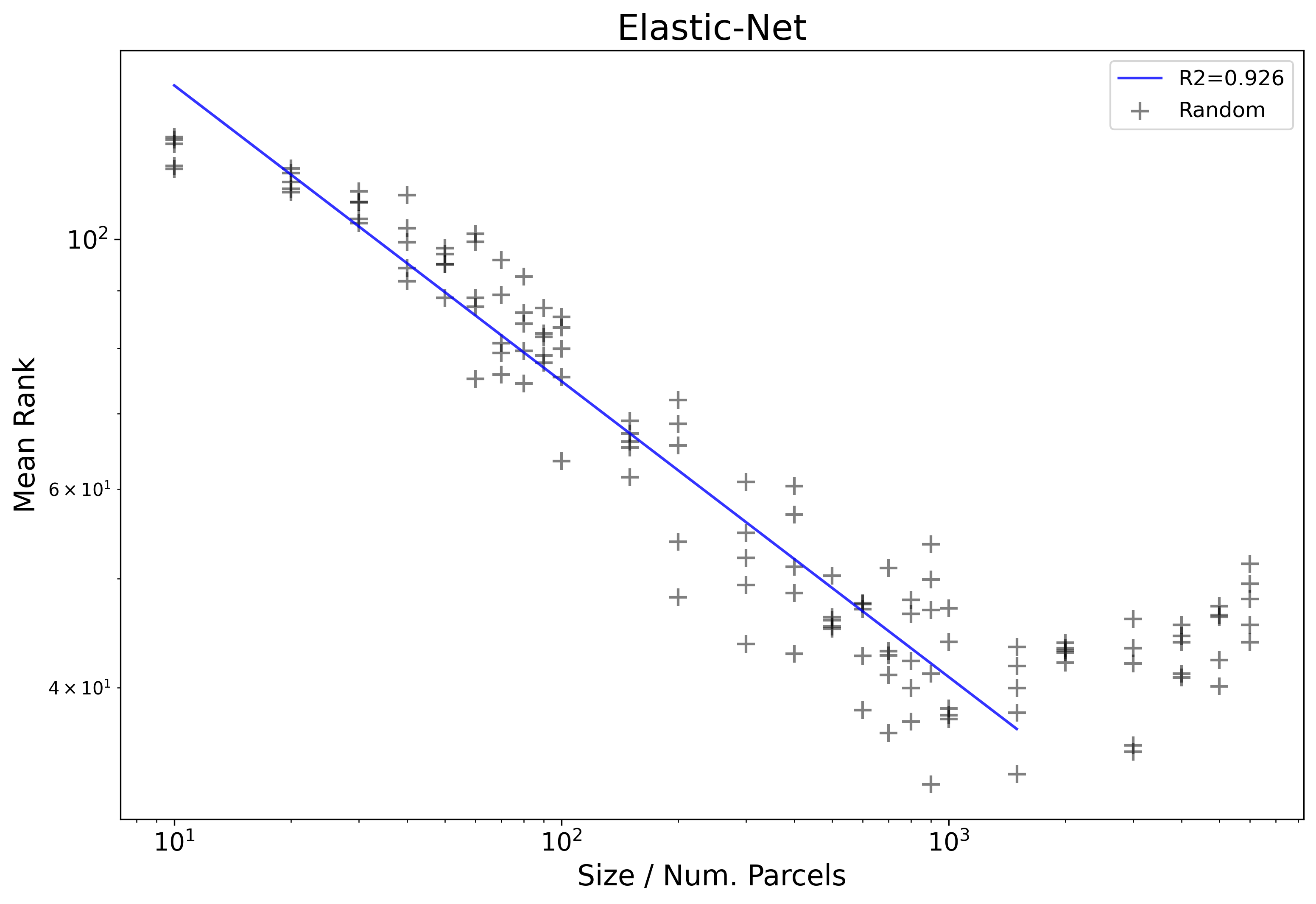
Next, we can consider an example plot showing real results from the core project experiment. In this example we will look at only results from the Elastic-Net based pipeline and from randomly generated parcellations.

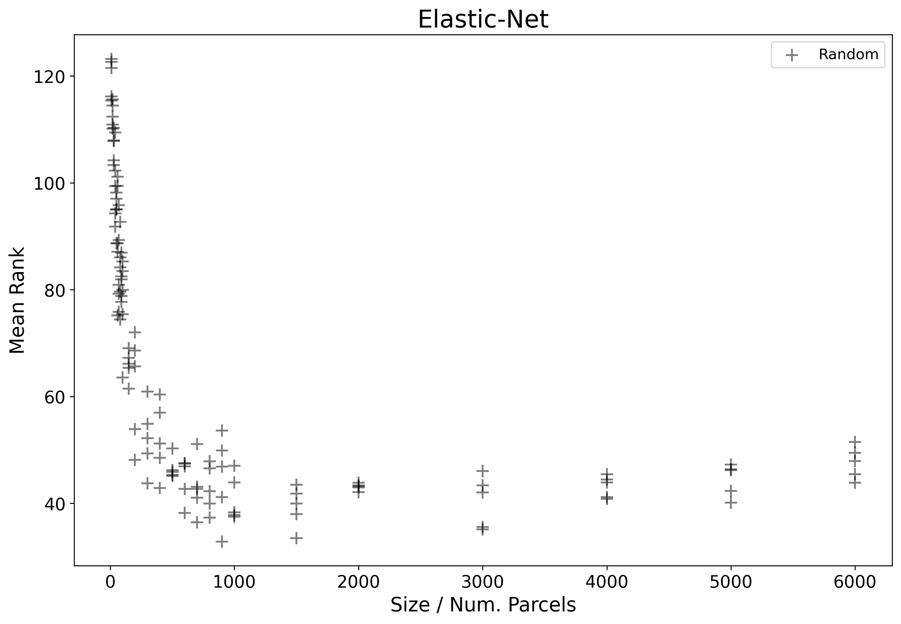
The x-axis here represents the number of parcels that each parcellation has, and the y-axis, the mean rank as computed by ranking each parcellation relative to all others plotted here for all 45 target variables.

Another useful way to view results is to re-create the same plot, but on a log-log scale.

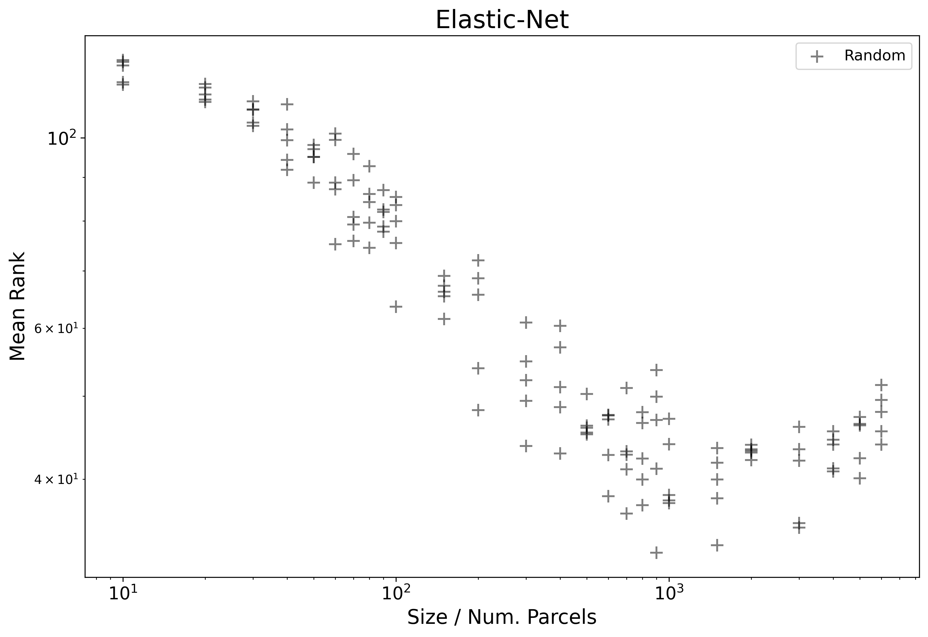
In this case we start to see a more clear traditional linear pattern emerge. In order to more formally model these results, we will first estimate the region where a powerlaw holds, then on this subset of data points (sizes 10-1500), fit a linear model as log10(Mean_Rank) ~ log10(Size):

OLS Regression Results

Dep. Variable:	Mean_Rank	R-squared:	0.926
Model:	OLS	Adj. R-squared:	0.925
Method:	Least Squares	F-statistic:	1288.
Date:	Tue, 16 Nov 2021	Prob (F-statistic):	4.98e-60

	coef	std err	t	P>|t|	[0.025	0.975]
Intercept	2.3989	0.017	142.937	0.000	2.366	2.432
Size	-0.2624	0.007	-35.883	0.000	-0.277	-0.248

We can also easily visualize the OLS fit onto the plot from before:

ML Pipeline Average Example

Lastly, we will update our definition of mean rank by now averaging across not just the 45 Target Variables, but also now across all three choices of ML Pipelines. Each plotted point below is now averaged from 135 different individually computed ranks.

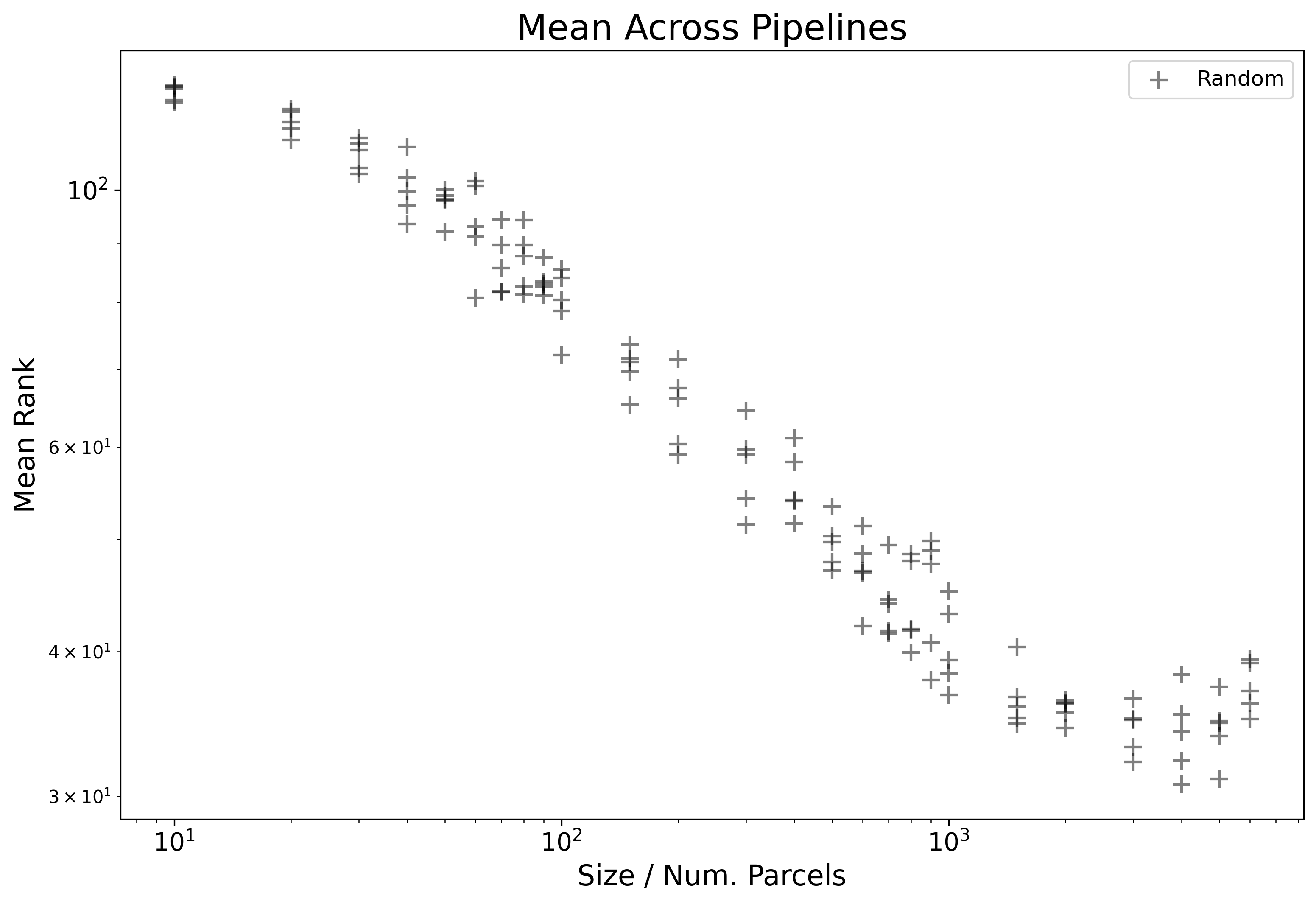
We can see here that by averaging now over pipeline too the linear pattern on the log-log plot becomes cleaner, and extends furthers. This is due to differences in performance across choice of pipeline.

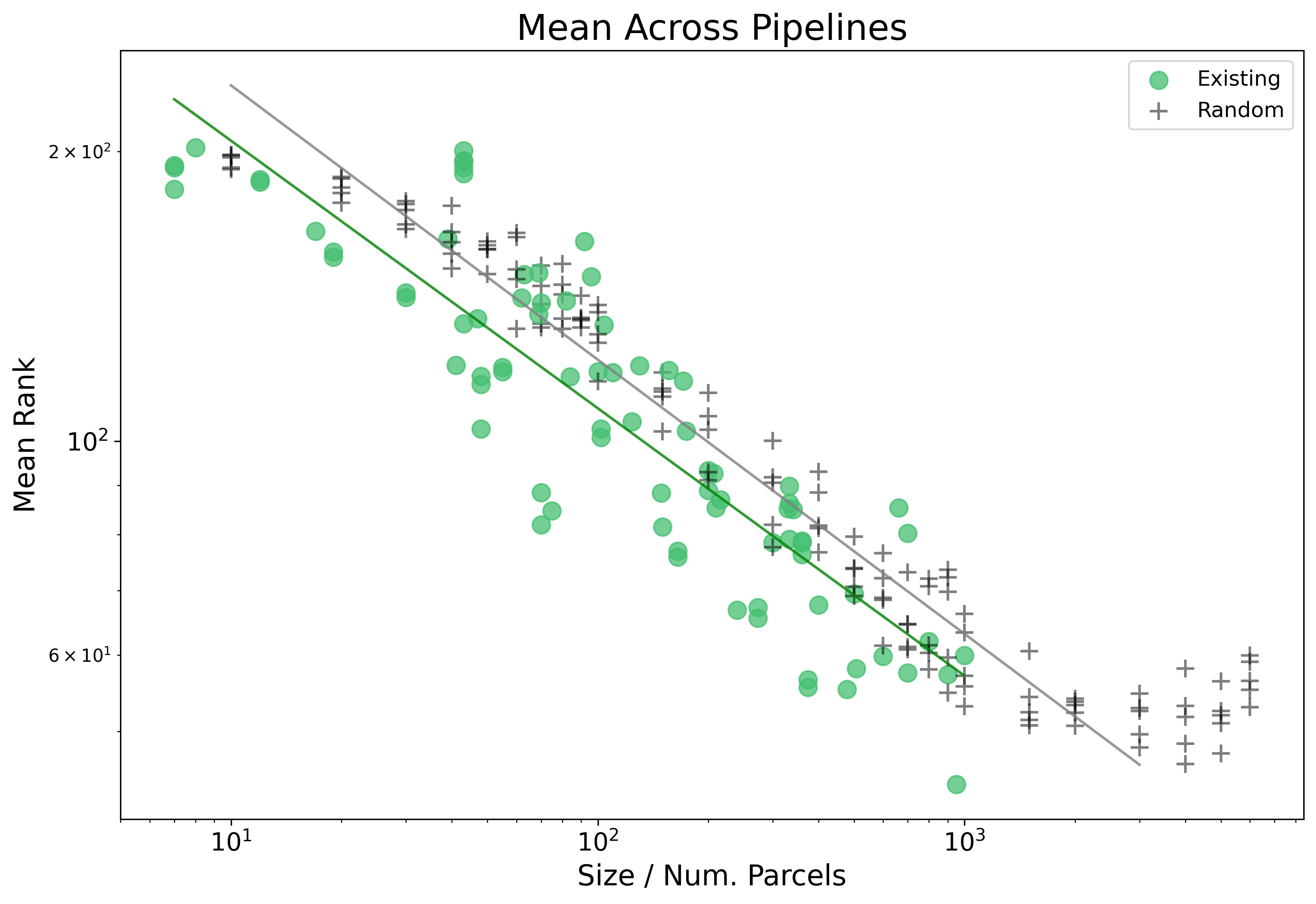
Model Choice of Parcellation Example

We can also add another layer of complexity, that is looking at more than one type of parcellation. We add in addition to random parcellations, existing parcellations:

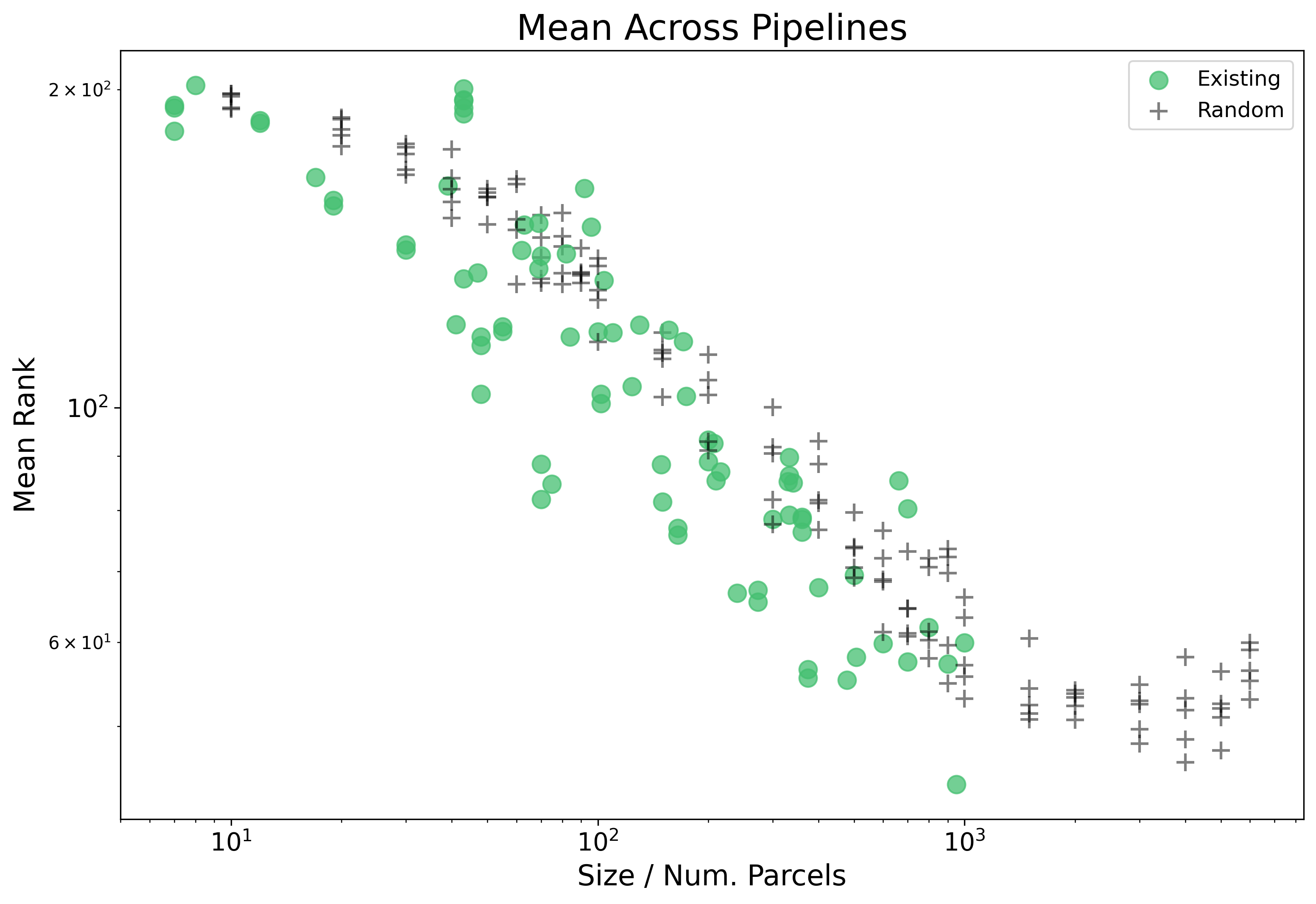
This also opens up another chance for modelling our results, where this time we can try and account for type of parcellation. First let’s model the results with type of parcellation as fixed effect, specifically: log10(Mean_Rank) ~ log10(Size) + C(Parcellation_Type)

OLS Regression Results

Dep. Variable:	Mean_Rank	R-squared:	0.895
Model:	OLS	Adj. R-squared:	0.893
Method:	Least Squares	F-statistic:	814.5
Date:	Tue, 16 Nov 2021	Prob (F-statistic):	1.61e-94

	coef	std err	t	P>|t|	[0.025	0.975]
Intercept	2.5993	0.016	164.374	0.000	2.568	2.630
C(Parcellation_Type)[T.Random]	0.0495	0.009	5.621	0.000	0.032	0.067
Size	-0.2824	0.007	-40.302	0.000	-0.296	-0.269

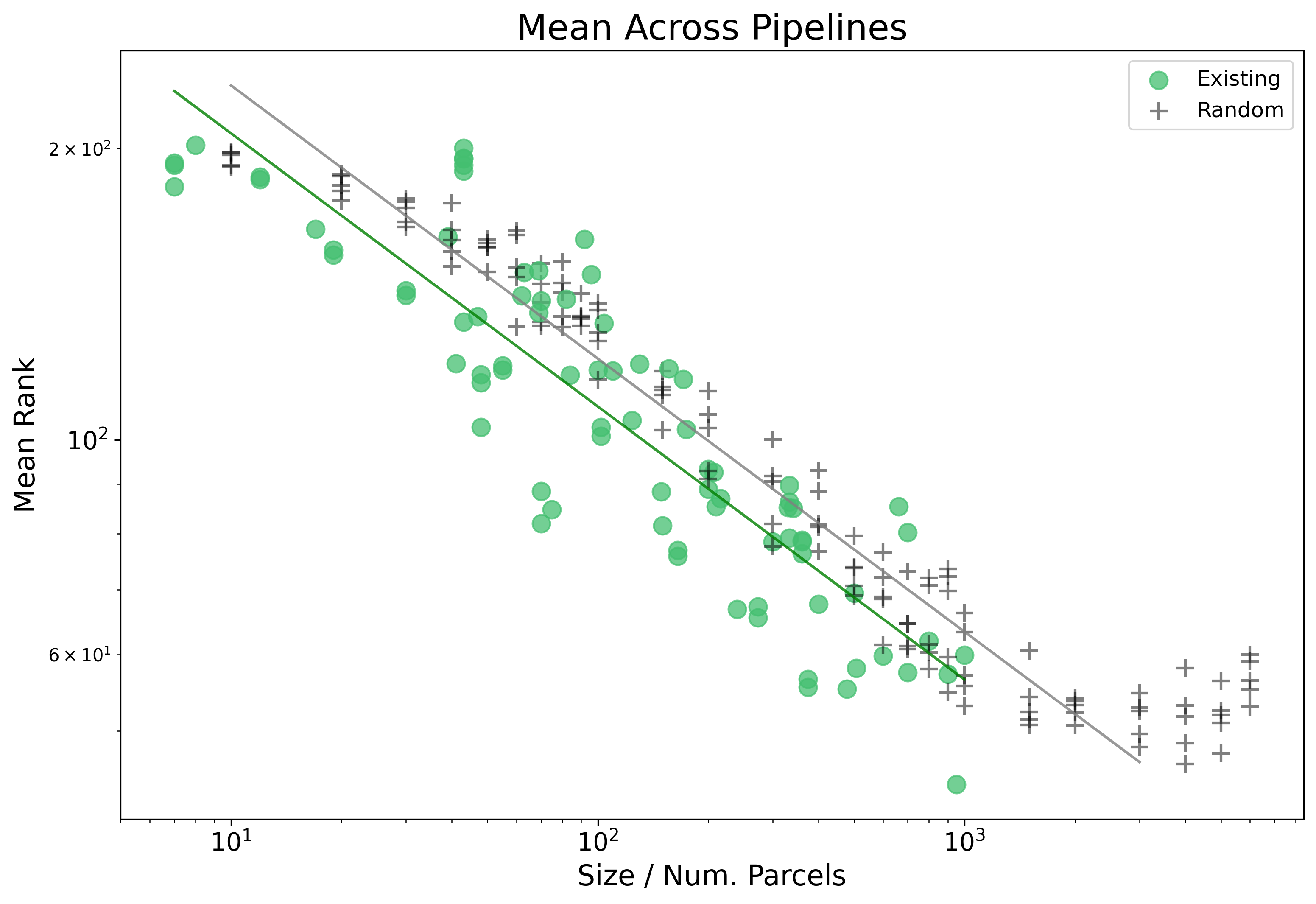
Noting above that the estimated range in which the distribution holds is up to size 2000, and that the the Existing parcellations get a boost to performance relative to their size.

Alternatively, we can choose to model Parcellation Type with a possible interaction as: log10(Mean_Rank) ~ log10(Size) * C(Parcellation_Type)

OLS Regression Results

Dep. Variable:	Mean_Rank	R-squared:	0.895
Model:	OLS	Adj. R-squared:	0.893
Method:	Least Squares	F-statistic:	540.9
Date:	Tue, 16 Nov 2021	Prob (F-statistic):	4.65e-93

	coef	std err	t	P>|t|	[0.025	0.975]
Intercept	2.5896	0.026	99.123	0.000	2.538	2.641
C(Parcellation_Type)[T.Random]	0.0644	0.033	1.942	0.054	-0.001	0.130
Size	-0.2777	0.012	-22.542	0.000	-0.302	-0.253
Size:C(Parcellation_Type)[T.Random]	-0.0070	0.015	-0.465	0.642	-0.037	0.023

We find no significant interaction with Size here, and can see in the plot below that the resulting fit is quite simmilar.