Results by Pipeline
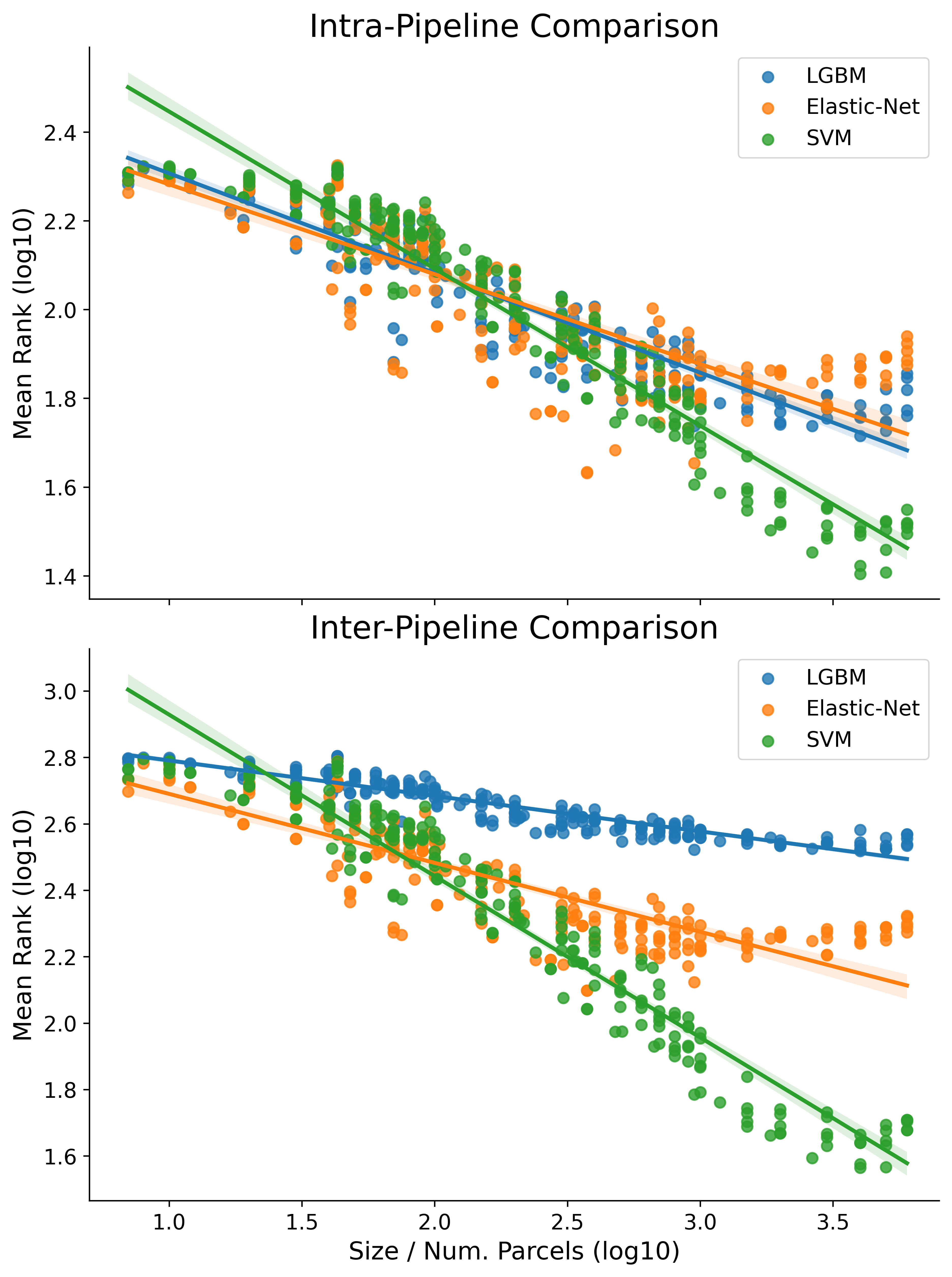
We break down the base results here by pipeline (instead of parcellation type) in two different ways: Intra and Inter pipeline (corresponding to the top and bottom of the figure below). If necessary first see the intro to results page for a guide on how the results in this project are interpreted.
-
The top part of the figure, Intra-Pipeline Comparison, shows mean rank for each pipeline as computed only relative to other parcellations evaluated with the same pipeline
-
The bottom part of the figure, Inter-Pipeline Comparison, shows mean rank as calculated between each parcellation-pipeline combination.
-
The regression line of best fit on the log10-log10 data are plotted separately for each pipeline across both figures (shaded regions around the lines of fit represent the bootstrap estimated 95% CI). The OLS fit here was with robust regression.
Intra-Pipeline Comparison
When comparing in an intra-pipeline fashion, we are essentially computing the ranks independently for each choice of ML Pipeline. We also estimate the powerlaw region separately for each.
- Elastic-Net: 7-2000
- SVM: 20-4000
- LGBM: 7-3000
We can then model these results as log10(Mean_Rank) ~ log10(Size) * C(Pipeline) where Pipeline
(the type of ML pipeline) is a fixed effect and can interact with Size (Fullscreen Plot Link).
| Dep. Variable: | Mean_Rank | R-squared: | 0.882 |
|---|---|---|---|
| Model: | OLS | Adj. R-squared: | 0.881 |
| Method: | Least Squares | F-statistic: | 878.8 |
| Date: | Mon, 03 Jan 2022 | Prob (F-statistic): | 2.48e-270 |
| coef | std err | t | P>|t| | [0.025 | 0.975] | |
|---|---|---|---|---|---|---|
| Intercept | 2.5893 | 0.019 | 135.246 | 0.000 | 2.552 | 2.627 |
| C(Pipeline)[T.LGBM] | -0.0208 | 0.026 | -0.795 | 0.427 | -0.072 | 0.031 |
| C(Pipeline)[T.SVM] | 0.3020 | 0.028 | 10.939 | 0.000 | 0.248 | 0.356 |
| Size | -0.2606 | 0.009 | -30.318 | 0.000 | -0.278 | -0.244 |
| Size:C(Pipeline)[T.LGBM] | 0.0162 | 0.012 | 1.405 | 0.160 | -0.006 | 0.039 |
| Size:C(Pipeline)[T.SVM] | -0.1291 | 0.012 | -10.957 | 0.000 | -0.152 | -0.106 |
The resulting statistical table is a little bit difficult to make sense of at first, so let’s also plot the fit to the data to get a better feel.
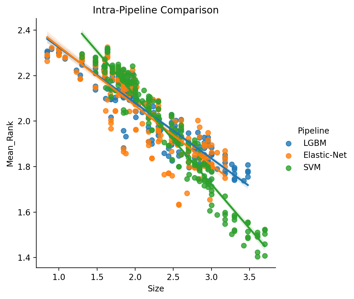
These results indicate that there are differences between the pipelines (i.e., scaling coefficient, range of scaling and intercept), as well as confirm more generally that scaling, albeit with varying degree, holds regardless of pipeline.
Another interesting way to view how results change when computed separately between pipelines is through an interactive visualization. Click Here for a fullscreen version of the plot.
A nice feature of the interactive plot is that by selecting different pipelines from the toggle, you can watch an animation of how specific results change with with different pipelines. You can also hover over specific data points to find out more information, for example what parcellation that data point corresponds to. You can also find a version of the interactive plot with non log10 axis here.
- Click here to see the full results table containing intra-pipeline specific results.
- See also Intra-Pipeline results as plotted by raw metric here
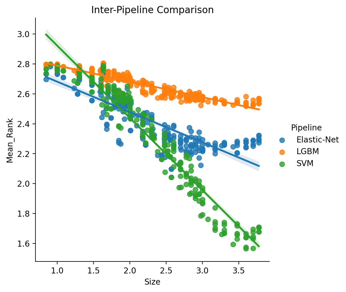
Inter-Pipeline Comparison
Alternately, we can compute rankings in an inter-pipeline manner, which means that the initial calculating of Rank is determined by directly comparing all Pipeline-Parcellation pairs for each target variable. The key difference here being inter-pipeline’s measure of mean rank as computed over 660 possible ranks versus intra as over 220 possible ranks.
We model these results in the same way as with the intra-pipeline comparison, but importantly using the different computation of mean rank. We also in this case do not estimate a powerlaw region of scaling as here we are more interested in the full statistical comparison. Formula: log10(Mean_Rank) ~ log10(Size) * C(Pipeline).
| Dep. Variable: | Mean_Rank | R-squared: | 0.921 |
|---|---|---|---|
| Model: | OLS | Adj. R-squared: | 0.921 |
| Method: | Least Squares | F-statistic: | 1527. |
| Date: | Mon, 03 Jan 2022 | Prob (F-statistic): | 0.00 |
| coef | std err | t | P>|t| | [0.025 | 0.975] | |
|---|---|---|---|---|---|---|
| Intercept | 2.8836 | 0.018 | 160.158 | 0.000 | 2.848 | 2.919 |
| C(Pipeline)[T.LGBM] | 0.0107 | 0.025 | 0.422 | 0.673 | -0.039 | 0.061 |
| C(Pipeline)[T.SVM] | 0.5203 | 0.025 | 20.432 | 0.000 | 0.470 | 0.570 |
| Size | -0.2026 | 0.007 | -27.342 | 0.000 | -0.217 | -0.188 |
| Size:C(Pipeline)[T.LGBM] | 0.0971 | 0.010 | 9.267 | 0.000 | 0.077 | 0.118 |
| Size:C(Pipeline)[T.SVM] | -0.2798 | 0.010 | -26.707 | 0.000 | -0.300 | -0.259 |
- Click here to see the full results table containing inter-pipeline specific results.
Extra
- See a recreation of these results but with Median Rank instead of Mean Rank here
- See also Inter/Intra Pipeline comparisons for ensembled results here
- How does front-end univariate feature selection influence scaling?
- See also Intra-Pipeline results as plotted by raw metric here