Results by Target

Importantly, by using mean rank, as the name implies we are taking the mean over all of the considered target variables. This is a useful strategy for reducing noise and making the results intelligible, but it can still be useful to look at the results as averaged only over choice of ML Pipeline. The below figure does exactly that:

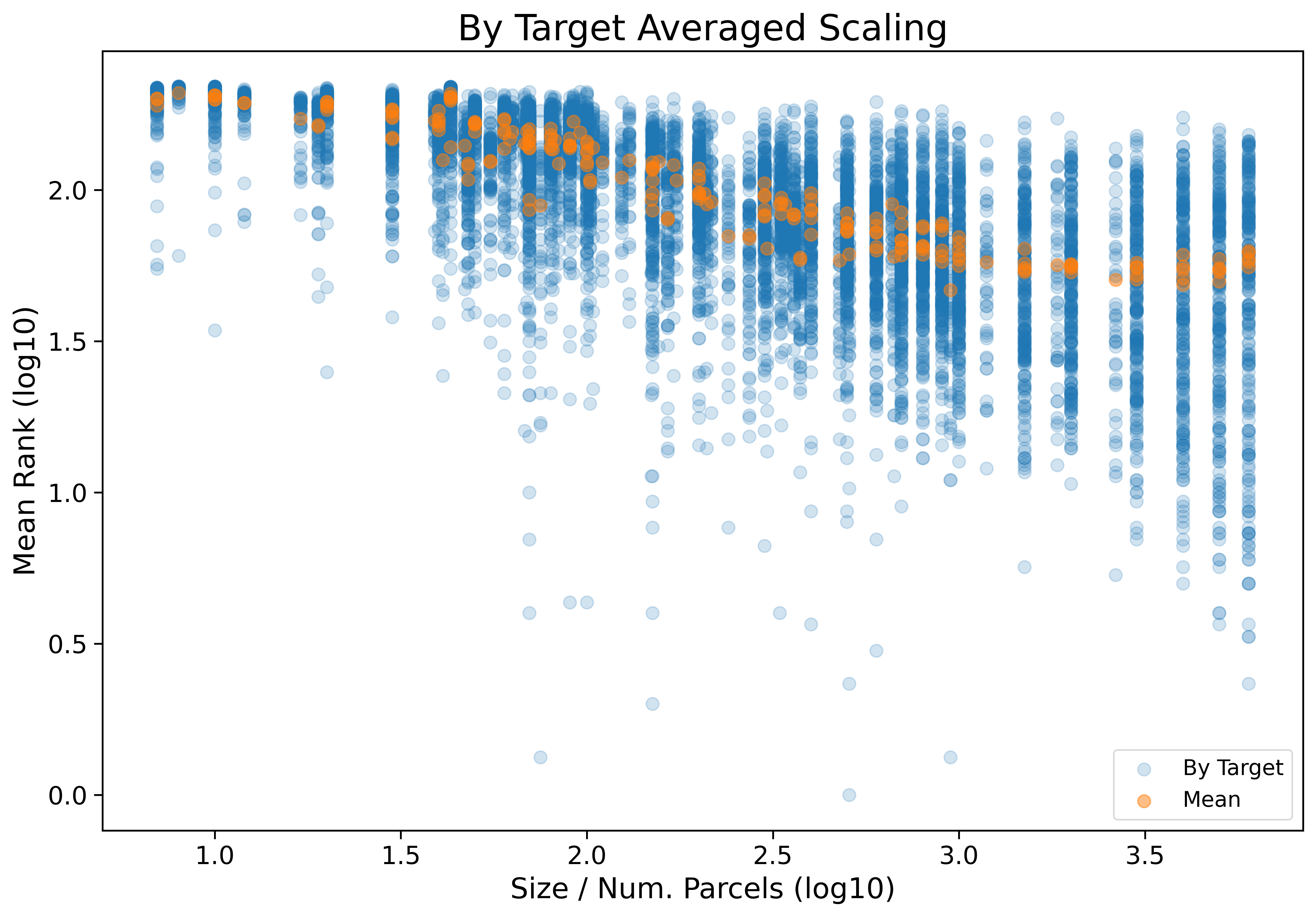
Click the figure above to open an interactive version of the plot. When using the interactive version of the plot it will be helpful to explore different plotly functionality for limiting the plot to just a subset of targets. To do this try double clicking on a target on the legend, this will isolate the plot to just that target variable. You can then add more by single clicking others, and eventually to reverse the isolation just double click twice on a target.

We can also look out what happens when we model these results, interested specifically in how our fit changes relative to just using the mean rank from the base results. Formula: log10(Mean_Rank) ~ log10(Size)

OLS Regression Results

Dep. Variable:	Mean_Rank	R-squared:	0.481
Model:	OLS	Adj. R-squared:	0.480
Method:	Least Squares	F-statistic:	9156.
Date:	Mon, 13 Sep 2021	Prob (F-statistic):	0.00

	coef	std err	t	P>|t|	[0.025	0.975]
Intercept	2.6315	0.007	360.421	0.000	2.617	2.646
Size	-0.2875	0.003	-95.690	0.000	-0.293	-0.282

Increasing Variance

Looking back at the main figure we notice another interesting thing. It appears like as sizes get bigger the spread of values also increases, such that the largest sizes may have the highest mean rank but they also have the highest variability. We can formalize this by computing the IQR at every unique size. We can then model this increasing spread as: IQR ~ log10(Size).

OLS Regression Results

Dep. Variable:	IQR	R-squared:	0.788
Model:	OLS	Adj. R-squared:	0.786
Method:	Least Squares	F-statistic:	283.2
Date:	Mon, 13 Sep 2021	Prob (F-statistic):	2.39e-27

	coef	std err	t	P>|t|	[0.025	0.975]
Intercept	-0.1946	0.024	-7.993	0.000	-0.243	-0.146
Size	0.1740	0.010	16.829	0.000	0.153	0.195

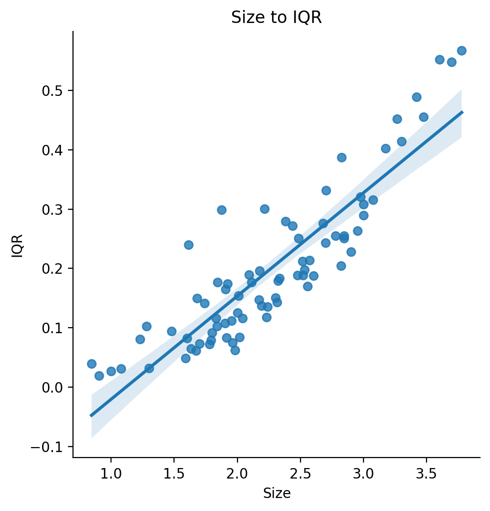
We actually end up with a pretty good fit explaining increase in IQR at each unique size from log10 of parcel size. One explanation for this is that increasing resolutions helps predict some target variables and not others. In this way, increasing resolution can improve performance on average, but will still sometimes not be a good fit.

Results Table

Click here to see the full and sortable raw results as broken down by target variable. Warning: this table is very large and difficult to make sense of, it may be easier to use the interactive plot.

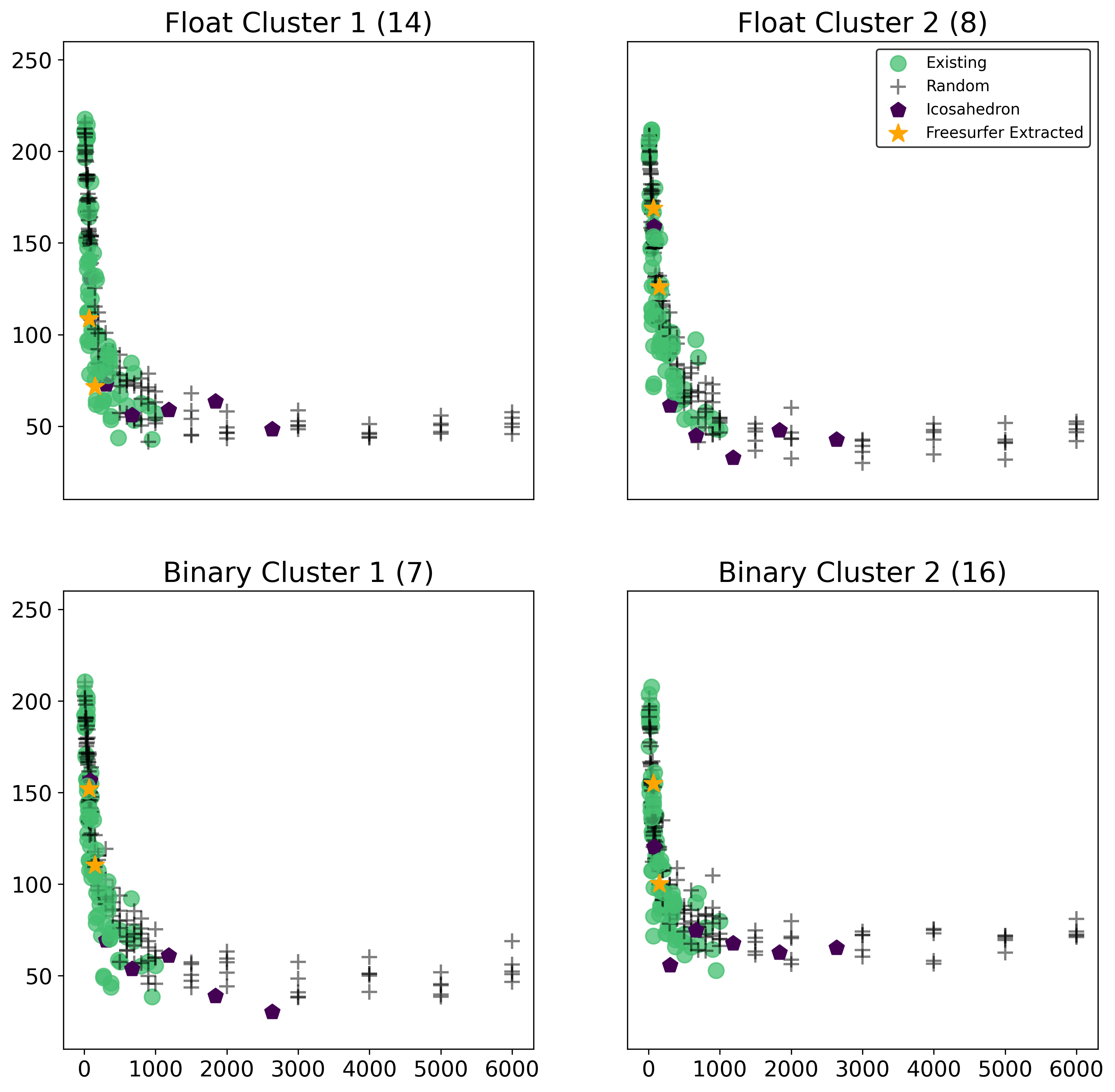
Results by Target Cluster

Another interesting way we can break down the results by targets is by first clustering the target variables in order to find groups which are simmilar. To do this, we use the scikit learn implementation of FeatureAgglomeration with linkage=’ward’. Note that clustering on targets is performed on only the subject of participants with no missing data for any of the target variables (7,894).

First we try a 4 clustering solution, where we perform clustering separately on the binary and continuous / float variable (2 clusters each), where clusters are:

Float Cluster 1:

[‘Parent Age (yrs)’, ‘Little Man Test Score’, ‘Neighborhood Safety’, ‘NeuroCog PCA1 (general ability)’, ‘NeuroCog PCA2 (executive function)’, ‘NeuroCog PCA3 (learning / memory)’, ‘NIH Card Sort Test’, ‘NIH List Sorting Working Memory Test’, ‘NIH Comparison Processing Speed Test’, ‘NIH Picture Vocabulary Test’, ‘NIH Oral Reading Recognition Test’, ‘WISC Matrix Reasoning Score’, ‘Summed Performance Sports Activity’, ‘Summed Team Sports Activity’]

Float Cluster 2:

[‘Standing Height (inches)’, ‘Waist Circumference (inches)’, ‘Measured Weight (lbs)’, ‘CBCL RuleBreak Syndrome Scale’, ‘Motor Development’, ‘Birth Weight (lbs)’, ‘Age (months)’, ‘MACVS Religion Subscale’]

Binary Cluster 1:

[‘Speaks Non-English Language’, ‘Months Breast Feds’, ‘Planned Pregnancy’, ‘Mother Pregnancy Problems’, ‘Parents Married’, ‘Sex at Birth’, ‘Sleep Disturbance Scale’]

Binary Cluster 2:

[‘Thought Problems ASR Syndrome Scale’, ‘CBCL Aggressive Syndrome Scale’, ‘Born Premature’, ‘Incubator Days’, ‘Has Twin’, ‘Distress At Birth’, ‘Any Alcohol During Pregnancy’, ‘Any Marijuana During Pregnancy’, ‘KSADS OCD Composite’, ‘KSADS ADHD Composite’, ‘Detentions / Suspensions’, ‘Mental Health Services’, ‘KSADS Bipolar Composite’, ‘Prodromal Psychosis Score’, ‘Screen Time Week’, ‘Screen Time Weekend’]

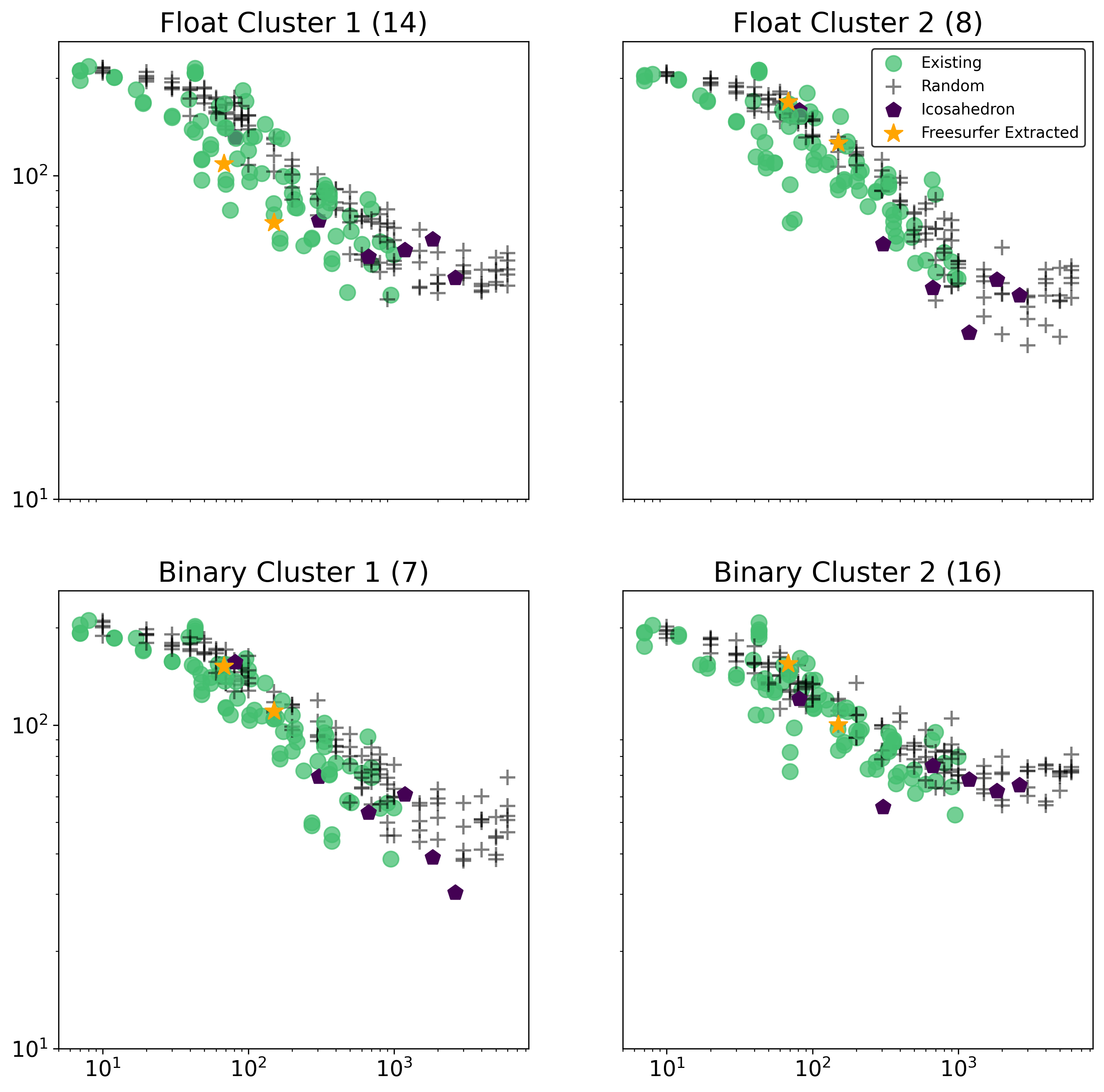
This subset is plotted below first on a normal scale, then on a log scale, where the mean ranks are determined from averaging just over the target variables in that cluster, and the number in ()’s refers to the number of variables in that cluster.

We can alternatively cluster over all of the target variables at once (ignoring if binary or not) with an adjustable number of clusters.

• See plots for 5 Clusters.
• See plots for 8 Clusters.
• See plots for 10 Clusters.
• See plots for 13 Clusters.

See Also

• See Regression Interactive By Target and Binary Interactive By Target .

• See All Interactive By Target to see a version of the interactive plot above, but with the results from the multiple parcellation strategies added as well.

• Likewise, see regression and binary version of the full interactive plots under All Regression Interactive By Target and All Binary Interactive By Target .

• Click here to see the full and sortable raw results as broken down by target variable, with the extra results from the multiple parcellation strategies added - though the interactive plot may be more legible.