Trade-Offs
Ultimately, in performing neuroimaging based machine learning, maximizing performance will typically not be the only consideration. Performance importantly has trade-offs with two other potentially key areas, namely interpretability and computational resources.
Interpretability
A natural benefit inherent in some existing parcellations is their popularity and widespread usage, which means named regions can be easily compared to prior literature employing that same atlas. For other parcellations, random or existing, it may instead require back-projecting feature importances to vertex surface space and interpreting values in this space. Similarly, instead of back-projecting feature importances, the parcellation itself can be automatically compared with a well known parcellation and region names assigned as combinations of well known regions.
Choice of pipeline will also influence how easily feature importances can be obtained, for example the Elastic-Net has associated beta weights and LGBM based pipeline a few different, although imperfect, measures of built in feature importance. The SVM based model though, since it employs the nonlinear radial basis function kernel, does not compute any built in measures of feature importance. Instead, a model-agnostic method must be used in order to derive feature importances. While these methods have their own trade-offs, there is certainly a growing interest in developing approaches to explain the outputs from “black-box” models (Altmann 2010, Lundberg 2017, Poyiadzi 2020).
Similar to the choice of pipeline is the choice of whether to ensemble over multiple parcellations. Where if an ensemble method is used, then interpretation is generally made more complex. However, for the voting ensemble, feature importances from the sub-model can be simply averaged, whereas for the stacking based ensemble a weighted average, according to the stacking models beta weights, can be used. In both cases, the use of permutation based feature importance can further be employed, allowing for the calculation of feature importances from base estimators without built in measures of importance. This idea is further expanded upon and implemented within the Python library Brain Predictability Toolbox (BPt). We provide an example jupyter notebook exploring in depth some of the different options for back projecting feature weights across all the different kinds of base estimators, ensembles, and parcellations considered in this project. An HTML version of this notebook is available here and the notebook itself can be found on the github here.
Runtime
The ML methods, atleast those used in this project, scale differently with respect to the number of input features. This scaling is therefore influenced by the the scale of the parcellations used as those with more parcels will produce more input feature and that will effect the computational resources needed to perform ML. We will consider in this section the influence of different parameters on runtime, noting of course that these times are with performance optimizations applied.
Caveat: In viewing plots of runtime it is important to remember that they may be biased in different ways given some of the quirks of the job submission system. For example, for parcellations with a small number of parcels, cluster jobs were typically submitted with lower resources and number of cores, therefore in the plot below where by plot only results run with 8 cores, it is important to keep in mind that most of the smaller parcellations were likely run with 4 or less cores.
The below plot shows violin plots of runtime as broken down by ML Pipeline on a subset of only jobs run with 8 cores and only jobs from the single parcellation base experiment. Parcellation size in the plot below is also rounded to the nearest 500.
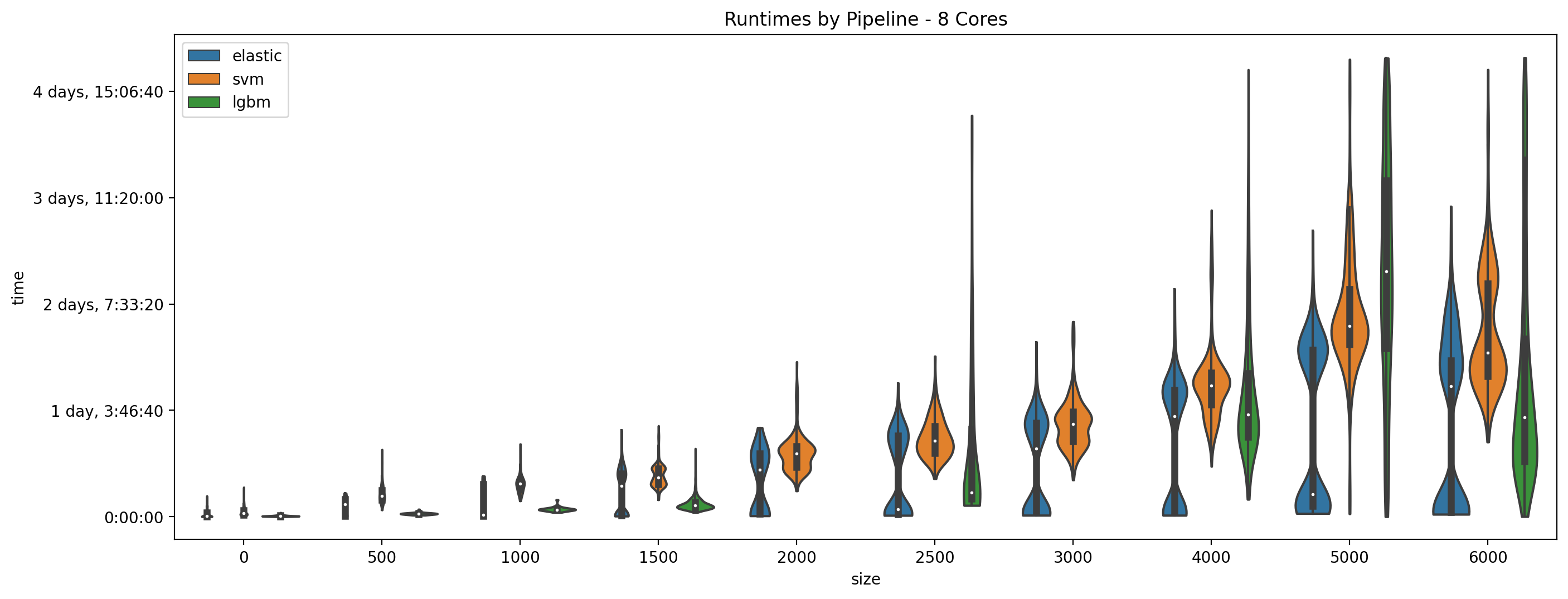
In general you will notice with this plot that parcellations with fewer parcels run much quicker, but also note that jobs with 8 cores were rarely used to run very small parcellations. The other interesting piece of this plots is how runtime changes based on the pipeline used, with the general pattern being Elastic-Net is quickest, followed by LGBM, then SVM. The Elastic-Net times are interesting though as they are bi-modal, this is because the binary version on average took longer than the regression version.
Contrast the 8-core jobs plot with the same plot but for only jobs run with 4 cores:
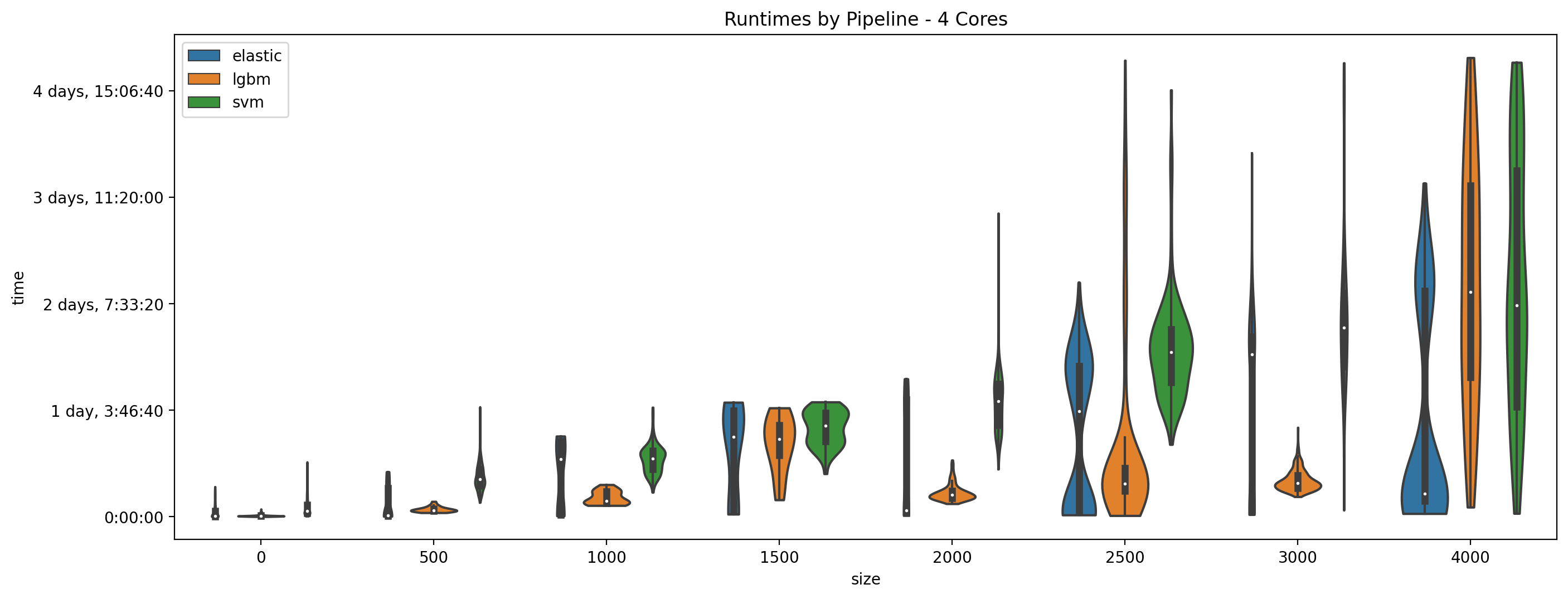
The jobs with 4 cores cut off at 4000, and as we can see the distribution extends all the way to the limit here. This indicates that these jobs took up to the maximum amount of time (up to 30 hours for each of the 5 folds.) We also notice an interesting pattern at sizes 1000 and 1500 where the distributions cut off suddenly at 30 hours. This is happens because parcellations at that size are submitted with all 5 folds in one job, so jobs that took longer than 30 hours just simply failed and were likely completed by a job with 8 or more cores instead.
Runtime for the Multiple Parcellation based strategies is more difficult to visualize due to extensive caching.
Upper Limit
There are also upper limits of runtime complexity to consider. We originally planned to run expiriments on the highest resolution data available, this is the vertex level data directly, but ultimately where unable to finish any of the expiriments (except the Elastic-Net based pipeline for regression targets only). The rest of the configurations, even running just a single of the 5 fold evaluations with up to 4 cores and up to 256GB of memory, were unable to complete within a week (the maximum time limit on the cluster) or failed due to memory constraints. The caveat here is that the algorithms and implementations we used were not necessarily designed for such high input data. If one were interested only in performing ML on vertex-wise data there are specially designed implementations of some algorithms which may be far more suitable. On the other hand, even if prioritizing performance, our current work shows that employing vertex-data directly may not even be necessary, as maximum performance (i.e., the end of the power law size scaling) can be reached with between 10^3 and 10^4 parcels.