Performance Optimizations

These expiriments were extremely computationally intensive to run, thus requiring a number of optimizations. Even just the base experiment required running 148,500 (220 parcellations * 45 targets * 3 pipelines * 5 evaluation folds) combinations! Which isn’t even considering the multiple parcellation strategies or that each of the pipelines hyper-parameter searches required training 180 different models…

The main overarching optimization / just thing that even made this at all possible was that the Vermont Advanced Computing Core was used to run all of the expiriments, which is a supercomputer. Even so, there are a number of other key / interesting optimizations made. This page will discuss some of the optimizations we made that allowed us to actually finish these expiriments / waste less resources.

Flexible Submission System

At first the idea of submitting jobs seems relatively easy, as essentially there are just a number of fixed configurations to run. We just need to run the submit.py file with all the choices of parcellation, model and target. Easy, just submit with 3 nested loops and done… except it turns out it isn’t nearly that simple.

The most fundamental problem relates to the different computational resources required by each combination. As it turns out, all three of the parameters of interest end up changing the resources needed, and all in different ways. The new problem we end up with is then how do we submit all of these different combinations, some of which can be run with a single core and a GB of memory in 10 minutes, and some of which will take 30 hours and 20+ GB just to run a single of the 5-folds?

The other points of interest when running these expiriments were runtime, that is to say getting results ASAP, and using as little resources as possible, as the cluster is a shared resource / using more resources hurts priority queue scores. Lastly, we were also interested in a system which required little to no manual intervention or babysitting.

The solution we built is based off of a randomized submission system. The core idea is that when a SLURM job is submitted, the first thing that job does is select a set of parameters (target, pipeline and parcellation) from a pool of options. This pool of options by default is just all of the remaining not finished options, but in order to add flexibility to different runtime consideration can be through passed input arguments set when submitting the job be used to restrict the pool of options in different ways (e.g., to just a specific pipeline).

This base randomized submission systems has a few really nice traits:

1. An arbitrary number of SLURM jobs can be submitted at any given time. Given that the cluster this was run on is shared by a number of other users, this was especially helpful as it let us submit large numbers of jobs during low usage times, and fewer jobs during periods of high use.

2. The system is flexible to failure. This is actually really important as ahead of time it is hard to know which configurations will fail. When a certain configuration fails though, it will be saved to an errors log and then just re-added to the pool of available jobs. In practice this means that without knowing ahead of time which jobs will fail, we could submit a first pass with a large number of low resource jobs. Then just a second pass with fewer high resource jobs that will end up processing only the ones that failed before as they will be all that are left unfinished. The key piece here is that we do not need to manually go in and check oh this specific job failed, then manually re-submit that job, etc… etc… instead we just continue to specify higher resource jobs.

Another aspect of the submission system which proved invaluable was a flag for certain parcellations with higher numbers of parcels. In this case these parcellation due to high numbers of input features would not be able to complete their 5-fold evaluation within a single 30 hour normal job. To solve this, we specified that these flagged parcellations would be submitted in an even more fine grained method, by-fold. These configurations were therefore added to the pool of options as not just choice of parcellation, pipeline and target but fold, and results saved for each fold by itself. This optimization proved sufficient for allowing us to run even very intensive expiriments, like parcellations with 6,000 parcels, using the same 30 hour default jobs. Likewise, using the flag method we were able to still save on the number of submitted jobs by still evaluating all five folds in one job for faster combinations of parameters!

Caching

Caching is a technique used in computer science in order to store results from intermediate computations and then when the same set of intermediate computations is encountered again, use the stored copy instead of re-computing the same set of instructions. Caching proved extremely useful in two key areas discussed below within this project.

Parcellation Caching

Extracting mean ROI values from data is fairly quick, maybe a bit longer for probabilistic parcellations. Notably in this project we use the same parcellations over and over, which means we then need to parcellate each subjects data over and over. For example take one of the existing parcellations in the base experiment, in this case the same parcellation needs to be applied for each combination of pipeline, target and for each of the 5-folds. The real bottle neck here though is the time it takes to load the raw (i.e., un-parcellated) data, especially using a cluster where the filesystem is very large and therefore slow.

All together it takes about 5-10 minutes to load just one combination of pipeline-target-fold, which means without any caching we would need to use the same repeated 5-10 minutes of loading 675 (3 pipelines * 45 targets * 5 folds) times for each parcellation. Given that we have 220 parcellations tested in the base experiment… you can start to see how big a waste of resources this might be if not handled - We are talking about around 12,000 hours of wasted computation (5min * 675 * 220).

Instead, we can cut that number down to just the initial 5-10 minutes for each parcellation, around 18 hours, so 675 times better. Specifically, we end up caching at the level of each participant-parcellation pair, such that only the first time a participants data is parcellated with a parcellation is the raw data loaded. Then every time a parcellation is needed for a specific participant the saved version is used instead. This caching is implemented through the Loader object via BPt.

Note: Another equivalently efficient method would be to pre-calculate the ROI values for all participant-parcellation pairs. It doesn’t really matter which way you go, though the two methods would require some changes to code structure and workflow.

Multiple Parcellation Strategy Caching

The multiple parcellation strategies require on the surface a huge, huge amount of computation. In order to ease this burden, we sought to as with the parcellation caching, make sure to set up the code to re-use intermediate results as much as possible.

Consider the diagram of different ensemble methods below:

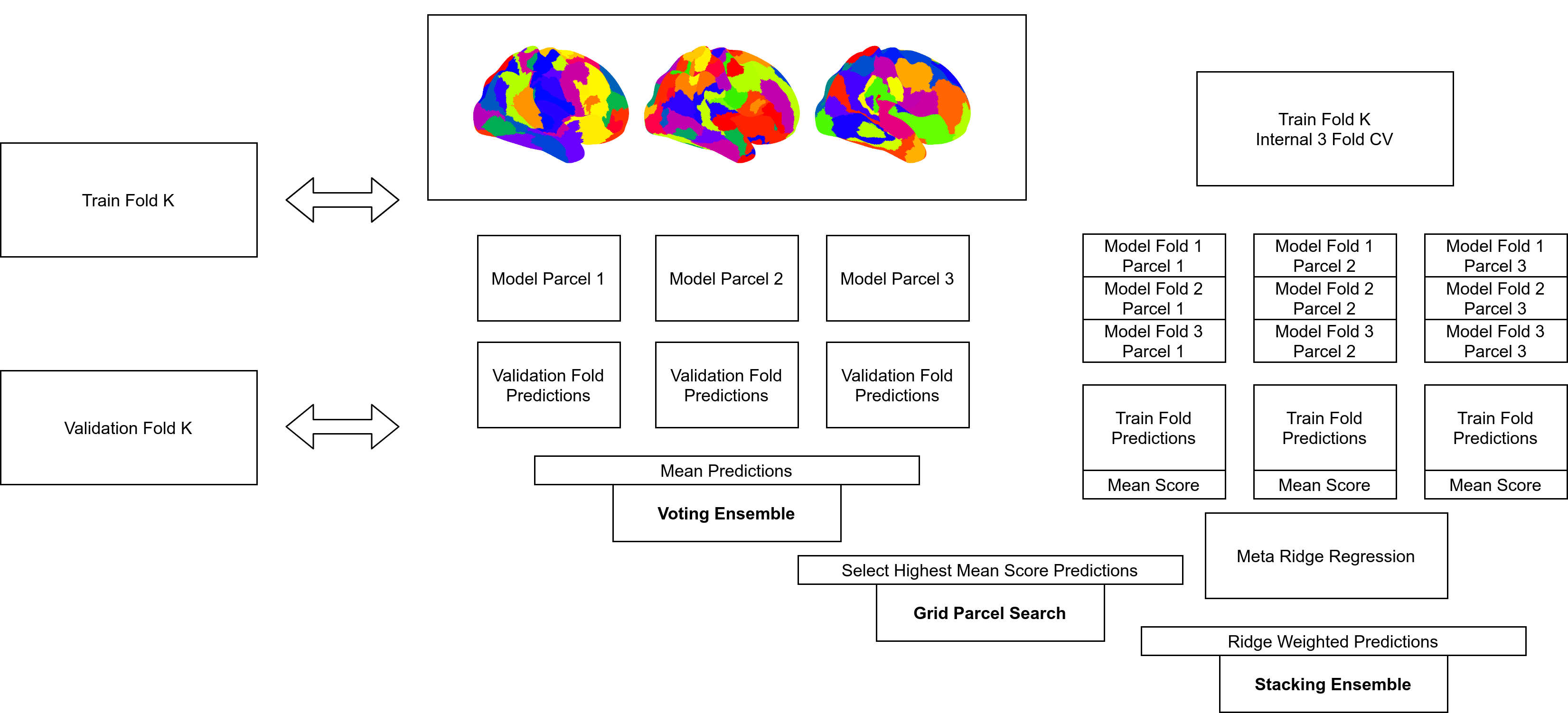
The important piece is that the base “Validation Fold Predictions” can be shared across all three multiple parcellation strategies, as they all require this information. Likewise, the internal three folder “Train Fold Predictions” can be shared across the “Grid” and “Stacked” strategies as in the grid search they are used to estimate performance and in the stacked strategy they are used to train a meta-estimator.

What this means is that we can setup caching specifically at the level of each of the pooled parcellations. Each parcellation in the pool then just needs to be fit 4 times (on the full training set and on the 3 internal folds of the training set), then those 4 fits re-used for each strategy.

By caching at the level of the individual parcellation within the pool of parcellations we receive another large benefit; that is, we can re-use intermediate results between runs. Consider first running a stacking ensemble on say 5 random parcellations each of size 100, once this is finished we now have cached results for each of these five random parcellations. So next when we run a stacking ensemble on 3 random parcellations of size 100, the cached results can be used and the full ensemble fit within minutes. Likewise, for the 8 random parcellations of size 100, we only need to train models for the 3 previously unseen parcellations. By setting up the caching this way and by re-using random parcellations we end up saving a large amount of computation.

Parallel Computing

It is common within ML implementations to be able to multi-process certain processes. This project was no exception, as we utilized heavily multi-processing (beyond the use of the cluster to submit multiple evaluation jobs at once) to parallelize primarily the hyper-parameter search within specific evaluation jobs.

Before this project we actually went in with some questions to test. Specifically, we wanted to know what the best strategy would be for running the huge amount of different ML expiriments described above, and not just that, but what would be the best use of parallel computing? The tricky part here is that there are an almost infinite number of different ways to slice it up. Given that each specific ML job can be parallelized, in terms of sometimes the base algorithm itself, or in this case in the hyper-parameter search, and also the different jobs themselves can be run at the same time given the SLURM computing cluster. So whats the best way to break it up?

One extreme would be to rely solely on the SLURM job level parallelization: basically every single ML job would just get one core to run on. This strategy has the benefit of 1. being easy to implement and 2. this type of single core job are the most readily available on the SLURM cluster used for this project. The big problem, and there is a big one, was that with just one core, each single job would take too long. Essentially if the job takes over 30 hours, then benefit number 2 is cancelled as jobs that take over 30 hours are very limited in supply.

The other extreme would be try to maximize parallelization within the job itself. Given searching over 60-180 hyper-parameters, and potential further parallelization we could with enough resources finish specific jobs very quickly. This though would require either requesting scarce very high resource computational nodes from the SLURM cluster or explored a distributed solution like dask distributed. We did explore dask distributed, the idea being to submit multiple lower resource jobs (avoiding the issue of node scarcity) and then set them up to be dask worker nodes, which can communicate with a master node that would run one ML job in a massively parallel way. In practice… we got it working, but only after a good amount of effort. This solution ended up requiring far too much over-engineering and in the end was not even competitive with the eventual strategy we landed upon, not to mention was filled with all sorts of very small but tricky edge cases (e.g., what if the main job starts running, but the worker jobs are still stuck on the queue… in this case the main job will just stall waiting to connect to the worker jobs).

So what did we end up doing? In the end we settled on a hybrid approach where we would submit nodes with somewhere between 1-16 cores, with the actual number depending on how long it takes for a certain parcellation-pipeline-target combination, e.g., if the job is short then we just submit a more readily available 1 core job, but if intensive need to submit up to a more scarce 16 core job. This allowed us parallelize both across jobs, submitting sometimes up to hundreds of jobs at once, and in a flexible way within job (using only as much resources as needed to finish within 30 hours).

It is also worth noting that the within job hyper-parameter parallelization we ended up using was with a joblib backend. To start we had been using python default multi-processing, but on the SLURM cluster it was extremely buggy, and sometimes jobs would just hang and not work for seemingly no reason (this was actually one of the reasons we first tries the dask distributed approach). Ultimately though, we ended up using the joblib code which was a true lifesaver and has been added as the new default in BPt!