Multiple Parcellation Strategies Setup
In addition to the base analysis, we sought to quantify how additional strategies operating across multiple parcellations might perform. Given a potentially limitless number of potential configurations, we explored only a small subset. We ultimately tested 3 different strategies: Grid, Voted and Stacked, which we explain later in more detail
Research Goals
Specific questions we sought to address included which multiple parcellation strategy, as well as which parcellations are included in that strategy, and how those choices influence performance. For example, how do the number of parcellations as well as the number of parcels in each parcellations contribute to performance gains. Should the included parcellations for any one ensemble be all of one fixed size or instead span across different sizes (e.g., five parcellations of size 300 each versus five parcellations with sizes 100, 200, 300, 400 and 500). Finally, how these different decisions influence trade-offs between performance, runtime and interpretability, is an important consideration.
Parcellations Used
In all of the multiple parcellation based analytic approaches, random parcellations were used as the source or “pool” of parcellations in which these strategies had access to. This choice was made as a virtually limitless number of random parcellations can be generated at any desired spatial scale. This flexibility makes them ideal for testing the different research goals of interest here.
Strategies
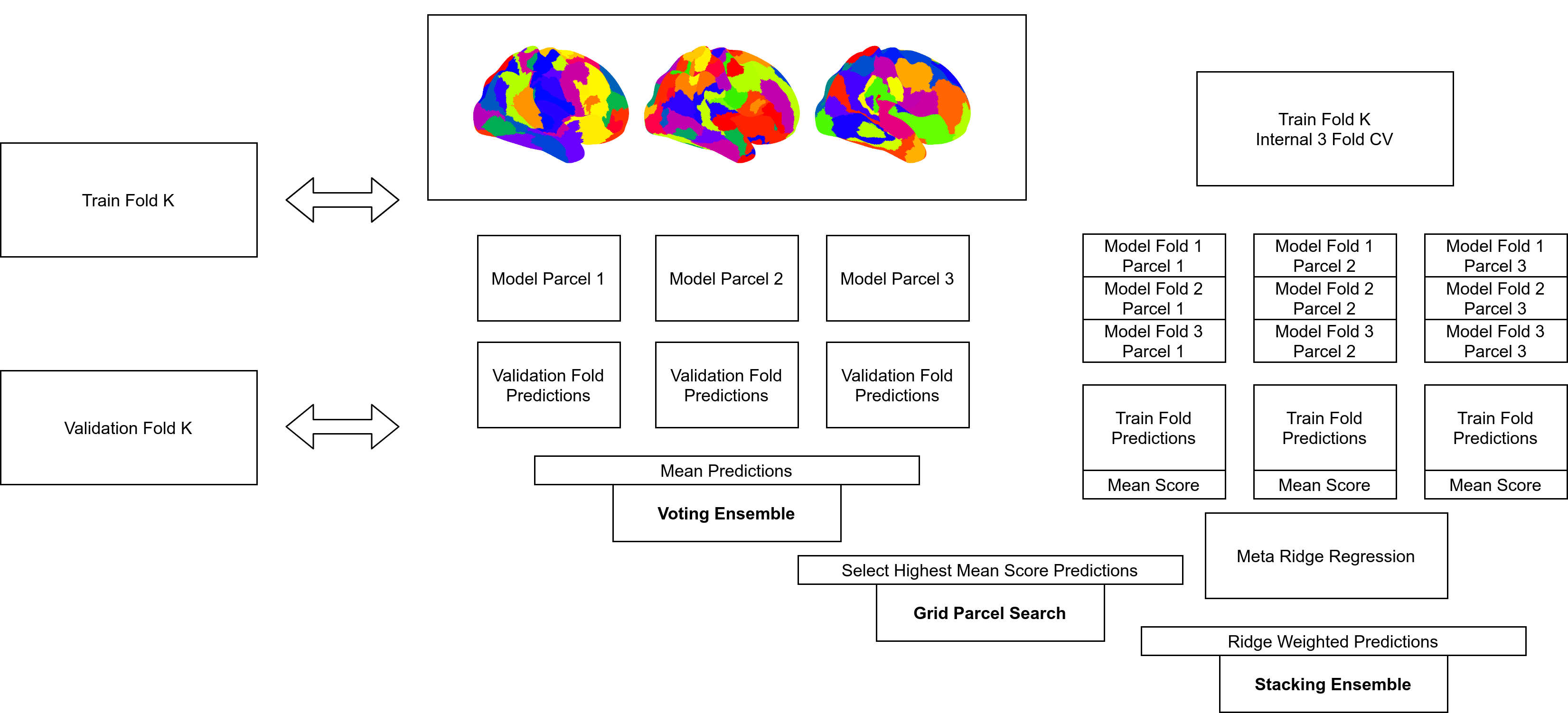
Grid
The “Grid” based strategy was designed to treat choice of parcellation as a hyperparameter. The motivation behind this idea being that nested cross validation could perhaps help to identify the best single parcellation from group of potential parcellations. In order to treat choice of parcellation as a hyperparameter, we employed a nested grid search. A three-fold nested cross-validation scheme on the training set, respecting family structure as before (i.e., assigning members of the same family to the same fold), was used to evaluate each potential parcellation. Within each of these internal folds a ML pipeline was trained, with its own nested parameter tuning, and then evaluated on its respective internal validation set. This process yielded an average for each of the three folds’ scores for each parcellation. The parcellation which obtained the highest score was selected for re-training on the full training set which involved, as in each nested fold, training a ML pipeline with its own nested parameter search. The final trained ML estimator, with the selected best parcellation, was then used to evaluate the validation fold. This process was repeated across the whole training set according to the same five-fold structure as used in the base analyses, thus allowing the results to be directly comparable.
Voted
The voting based strategy is the simpler of the ensemble based strategies tested. In this approach, a separate estimator was trained for each available parcellation, where each individual pipeline-parcellation pair was trained in the same way as in the base analysis. To do this, first each trained ML pipeline from the previous step generated a prediction. Then, the voting ensemble aggregated the predictions as either the mean, in the case of regression, or the most frequently predicted class, in the case of classification. The aggregated scores were then scored as a single set of predictions.
This approach was based on implementations of the voting classifier and voting regressor in scikit-learn, the final version making use of the BPt tweaked versions. The ‘estimators’ in this case, the base models to be averaged, are separate versions of the same base ML pipeline but trained on features as extracted from different random parcellations.
Stacked
The stacking ensemble, while similar to the voting ensemble, is a bit more complex. For each of the pipeline-parcellation combinations, a separate three-fold cross-validation framework was used in the training set. In this framework, three ML pipelines were trained on 2/3 of the training set and predictions were made on the remaining 1/3, yielding an out-of-sample prediction for each participant in the training set (notably this is the same nested three fold validation used in the grid strategy). The predictions from all pipeline-parcellation combinations were used as features to train a “stacking model”. The purpose of the stacking model was to learn a relative weighting of each parcellation-pipeline combination (i.e., to give more weight to better parcellation-pipeline combinations and less weight to worse ones). The algorithm used to train the stacking model was a ridge penalized linear or logistic regression with nested hyper-parameter tuning. Once trained, this stacking model was used to predict the target variable in a novel sample (i.e., the held-out test set). The stacking ensemble procedure notably involved a large increase in computation relative to the voting ensemble, as the stacking ensemble involved training three pipelines for each parcellation-pipeline combination, whereas the voting ensemble consisted of training only one ML pipeline for each.
This approach was based on the scikit learn implementation of stacked generalization, as ultimately implemented in BPt. Like with the voting based strategy, the key detail here is the base models used for stacking were separate versions of the same base ML pipelines but trained on features as extracted from different random parcellations.
Evaluation
Each considered multiple parcellation strategy was evaluated in a directly comparable way to the base analysis (i.e., for each target with the same five-fold cross-validation - Read More). As in the base analysis, multiple parcellation analyses were first run for each choice of ML pipeline separately. Additionally, we also considered a special ‘All’ configuration, ensembling and selecting across both parcellation and choice of ML pipeline (e.g., a voting ensemble which averages predictions from SVM, Elastic-Net and LGBM pipelines, each trained on random parcellations of size 100, 200 and 300).
For the number of different parcellations available to a search or ensemble strategy, we evaluated four different numbers of parcellations: 3, 5, 8 and 10. Further, for each of these numbers of parcellations, we tested fixed size parcellations as well as differentially sized parcellations across a range of sizes (100, 200, 300, 400, 500, 50-500, 100-1000 and 300-1200). For example, for a combination of 3 parcellations and a fixed size of 100, three random parcellations with size 100 could be used. For a combination of 5 parcellations of a range of sizes from 100-1000, parcellations of size 100, 325, 550, 775 and 1000 could be used. All combinations are then repeated twice with two different versions of parcellations at each size used.
Ultimately, all combinations of the following parameters were evaluated:
8 Size Configurations (5 Fixed Sizes + 3 Across Sizes)4 Number of Parcellations (3, 5, 8, 10)3 Base Strategies (Grid, Voted, Stacked)4 Pipelines (3 Base Pipelines + 'All' Configuration)45 Target Variables2 Random Repeats
In total: 34,560 combinations.
On Naming
Within the results sections on this site these multiple parcellation strategies are referenced with names like: “stacked random 500 10 0”. In this example this means this was a stacking based ensemble comprised of 10 random parcellations all of size 500. Lastly the 0 at the end refers to the repeat (i.e., there is another result called “stacked random 500 10 1” that was also a stacking based ensemble of 10 random parcellations all of size 500, but a different 10 random parcellations).Likewise, if voting or grid based then names would be “voted random 500 10 0” and “ “grid random 500 10 0” respectively.
The across sizes variant is simmilar, but maybe a bit confusing. For example if the name is “voted random 100 1000 10 0”, then that means it was a voting based ensemble with 10 random parcellations ranging in size from 100 to 1000 (in this case sizes 100, 200, 300, 400, 500, 600, 700, 800, 900, 1000).
Lastly, in section Special Ensembles there is an additional variation where names can be listed under stacked and then a special keyword referring to a collection of existing parcellations. For example “stacked schaefer” refers to a stacking ensemble over all of the the 10 Schaefer Parcellations.
Implementation
The implementation for these different ensemble methods is contained within the same file where the different pipelines are defined, in exp/models.py, using code from BPt version 2.0+.
One key implementation detail is that the different multiple parcellation strategies were designed with maximum reusability in mind via an extensive caching system. To read more in depth about this important optimization see Optimizations: Multiple Parcellation Strategy Caching.