Predict BMI#

This script shows a real world example using BPt to study the relationship between BMI and the brain. The data used in this notebook cannot be made public as it is from the ABCD Study, which requires a data use agreement in order to use the data.

This notebook covers a number of different topics:

Preparing Data
Evaluating a single pipeline
Considering different options for how to use a test set
Introduce and use the Evaluate input option

[1]:

import pandas as pd
import BPt as bp
import numpy as np

# Don't show sklearn convergence warnings
from warnings import simplefilter
from sklearn.exceptions import ConvergenceWarning
simplefilter("ignore", category=ConvergenceWarning)

# Display tables up to five decimals
pd.options.display.float_format = "{:,.5f}".format

Preparing Data#

We will first load in the underlying dataset for this project which has been saved as a csv. It contains multi-modal change in ROI data from two timepoints of the ABCD Study (difference from follow up and baseline).

This saved dataset doesn’t include the real family ids, but an interesting piece of the ABCD study derived data is that there are a number of subjects from the same family. We will handle that in this example (granted with a fake family structure which we will generate below) by ensuring that for any cross-validation split, members of the same family stay in the same training or testing fold.

[2]:

data = pd.read_excel('data/structure_base.xlsx')
list(data)[:10]

[2]:

['Unnamed: 0',
 'src_subject_id',
 'b_averaged_puberty',
 'b_agemos',
 'b_sex',
 'b_race_ethnicity_categories',
 'b_demo_highest_education_categories',
 'b_site_id_l',
 'b_subjects_no_missing_data',
 'bmi_keep']

This dataset contains a number of columns we don’t need. We will use the next cell to both group variables of interest together, and then select only the relvant columns to keep.

[3]:

# Our target variable
targets = ['b_bmi']

# Columns with different traditional 'co-variates'.
covars = ['b_sex',  'b_demo_highest_education_categories','b_race_ethnicity_categories',
          'b_agemos', 'b_mri_info_deviceserialnumber']

# Let's also note which of these are categorical
cat_covars = ['b_mri_info_deviceserialnumber',
              'b_demo_highest_education_categories',
              'b_race_ethnicity_categories',
              'b_sex']

# These variables are any which we might want to use
# but not directly as input features! E.g., we
# might want to use them to inform choice of cross-validation.
non_input = ['b_rel_family_id']

# The different imaging features
thick = [d for d in list(data) if 'thick' in d]
area = [d for d in list(data) if 'smri_area_cort' in d]
subcort = [d for d in list(data) if 'smri_vol' in d]
dti_fa = [d for d in list(data) if 'dmri_dti_full_fa_' in d]
dti_md = [d for d in list(data) if 'dmri_dti_full_md_' in d]
brain = thick + area + subcort + dti_fa + dti_md

# All to keep
to_keep = brain + targets + covars + non_input

data = data[to_keep]
data.shape

[3]:

(9724, 668)

Now let’s convert from a pandas DataFrame to a BPt Dataset.

[4]:

data = bp.Dataset(data)

# This is optional, to print some extra statements.
data.verbose = 1
data.shape

[4]:

(9724, 668)

Next, we perform some actions specific to the Dataset class. These include specifying which columns are ‘target’ and ‘non input’, with any we don’t set to one these roles treated as the default role, ‘data’.

[5]:

# Set's targets to target role
data = data.set_role(targets, 'target')

# Set non input to non input role
data = data.set_role(non_input, 'non input')

# Drop any missing values in the target variable
data = data.drop_subjects_by_nan(scope='target')

# We can optional add the categories we made as scopes!
data.add_scope(covars, 'covars', inplace=True)
data.add_scope(cat_covars, 'cat covars', inplace=True)
data.add_scope(thick, 'thick', inplace=True)
data.add_scope(area, 'area', inplace=True)
data.add_scope(subcort, 'subcort', inplace=True)
data.add_scope(dti_fa, 'dti_fa', inplace=True)
data.add_scope(dti_md, 'dti_md', inplace=True)
data.add_scope(brain, 'brain', inplace=True )

# Drop all NaN from any column
# Though BPt can generally handle NaN data fine,
# it makes certain pieces easier for this example as we don't have to worry
# about imputation.
data = data.dropna()

# Just show the first few rows
data.head()

Setting NaN threshold to: 0.5
Dropped 8 Rows

[5]:

Data

	b_agemos	b_demo_highest_education_categories	b_mri_info_deviceserialnumber	b_race_ethnicity_categories	b_sex	dmri_dti_full_fa_subcort_aseg_accumbens_area_lh	dmri_dti_full_fa_subcort_aseg_accumbens_area_rh	dmri_dti_full_fa_subcort_aseg_amygdala_lh	dmri_dti_full_fa_subcort_aseg_amygdala_rh	dmri_dti_full_fa_subcort_aseg_caudate_lh	...	smri_vol_scs_subcorticalgv	smri_vol_scs_suprateialv	smri_vol_scs_tplh	smri_vol_scs_tprh	smri_vol_scs_vedclh	smri_vol_scs_vedcrh	smri_vol_scs_wholeb	smri_vol_scs_wmhint
0	124	2	HASHe4f6957a	2	1	0.17195	0.17389	0.19923	0.16654	0.15518	...	52,440.00000	935,475.83514	6,220.90000	5,787.40000	3,554.80000	3,427.90000	1,045,923.63514	478.40000
1	122	5	HASH1314a204	1	2	0.16897	0.16477	0.20000	0.17713	0.15848	...	62,550.00000	1,078,644.86257	8,222.60000	7,571.40000	3,872.50000	3,837.40000	1,197,394.06258	769.70000
2	114	3	HASH69f406fa	1	1	0.22881	0.25250	0.23221	0.22298	0.22545	...	60,695.00000	1,133,471.50460	7,040.50000	6,752.90000	4,588.80000	4,631.50000	1,291,126.70460	1,114.70000
3	130	5	HASH1314a204	1	2	0.16737	0.18840	0.15135	0.16215	0.18848	...	65,614.00000	1,055,580.45187	8,365.70000	7,656.40000	4,600.10000	4,920.60000	1,189,841.05187	1,788.50000
4	115	5	HASHc3bf3d9c	1	2	0.18902	0.21375	0.23945	0.20581	0.20100	...	59,174.00000	1,010,567.33270	6,577.90000	6,612.70000	3,434.30000	3,942.60000	1,144,069.73270	1,036.30000

5 rows × 666 columns

Target

	b_bmi
0	15.17507
1	16.45090
2	24.43703
3	17.38701
4	17.59670

Non Input

	b_rel_family_id
0	2257
1	11328
2	7607
3	11324
4	7608

The scopes we defined are nice, as it lets use check columns, or compose different scopes together. For example we can check the scope we set ‘cat covars’ as composed with another variable as:

[6]:

data.get_cols([cat_covars, 'b_rel_family_id'])

[6]:

['b_demo_highest_education_categories',
 'b_mri_info_deviceserialnumber',
 'b_race_ethnicity_categories',
 'b_rel_family_id',
 'b_sex']

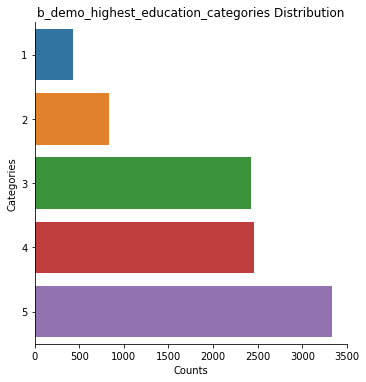
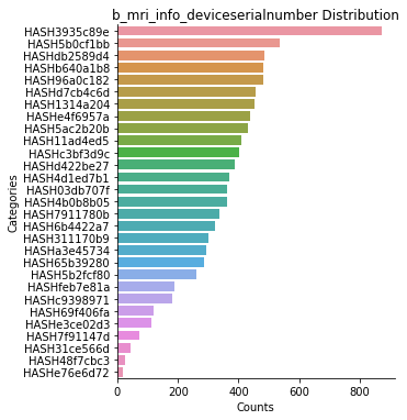
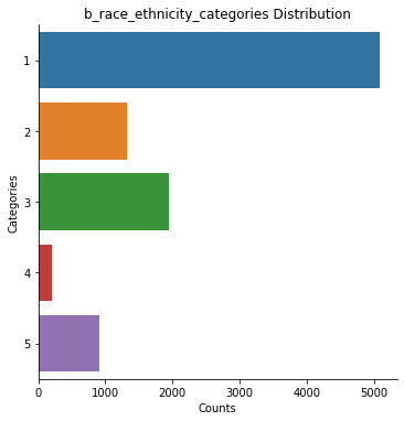
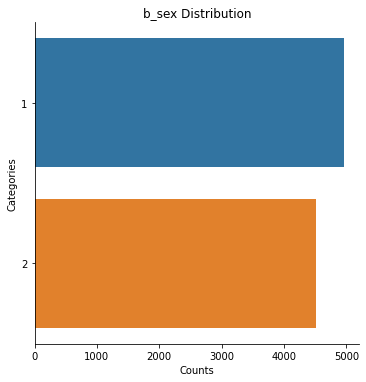
These are notably the columns we want to make sure are categorical, so lets ordinalize them, then plot.

[7]:

data = data.ordinalize([cat_covars, 'b_rel_family_id'])

# Then plot just the categorical variables
data.plot(scope='category', subjects='all', decode_values=True)

b_demo_highest_education_categories: 9478 rows

../_images/user_guide_bmi_full_example_14_1.png

b_mri_info_deviceserialnumber: 9478 rows

../_images/user_guide_bmi_full_example_14_3.png

b_race_ethnicity_categories: 9478 rows

../_images/user_guide_bmi_full_example_14_5.png

b_rel_family_id: 9478 rows
b_sex: 9478 rows

/home/sage/anaconda3/envs/bpt/lib/python3.9/site-packages/BPt/dataset/helpers.py:167: UserWarning: Skipping plot: b_rel_family_id as >= categories!
  warnings.warn(as_str)

../_images/user_guide_bmi_full_example_14_8.png

Let’s plot the target variables as well.

[8]:

data.plot('target')

b_bmi: 9478 rows

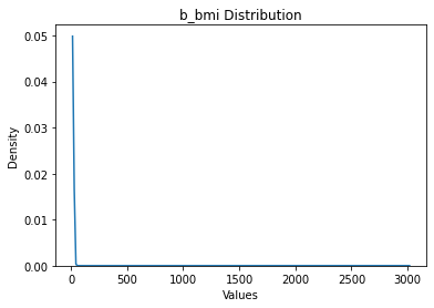
../_images/user_guide_bmi_full_example_16_1.png

Okay, we note that there are some extreme outliers.

[9]:

data = data.filter_outliers_by_std(n_std=10, scope='target')
data['target'].max()

Dropped 1 Rows

[9]:

b_bmi   53.90845
dtype: float64

[10]:

data.plot('target')

b_bmi: 9477 rows

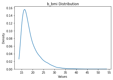
../_images/user_guide_bmi_full_example_19_1.png

Okay this maximum seem much more reasonable. Let’s also assume that there may be some extreme values present in the input data as well, and that these represet corrupted data that we therefore want to drop.

[11]:

# Repeat it twice, to deal with outliers at multiple scales
data = data.filter_outliers_by_std(n_std=10, scope='float')
data = data.filter_outliers_by_std(n_std=10, scope='float')

Dropped 62 Rows
Dropped 14 Rows

Next, we consider splitting up out data with a global train and test split. This can be useful in some instances. Note that we also define a cv strategy which says to perform the train test split keeping members of the same family in the same fold.

[12]:

# Let's say we want to keep family members in the same train or test split
cv_strategy = bp.CVStrategy(groups='b_rel_family_id')

# Test split
data = data.set_test_split(.2, random_state=5, cv_strategy=cv_strategy)
data

Performing test split on: 9401 subjects.
random_state: 5
Test split size: 0.2

Performed train/test split
Train size: 7481
Test size:  1920

[12]:

Data

	b_agemos	b_demo_highest_education_categories	b_mri_info_deviceserialnumber	b_race_ethnicity_categories	b_sex	dmri_dti_full_fa_subcort_aseg_accumbens_area_lh	dmri_dti_full_fa_subcort_aseg_accumbens_area_rh	dmri_dti_full_fa_subcort_aseg_amygdala_lh	dmri_dti_full_fa_subcort_aseg_amygdala_rh	dmri_dti_full_fa_subcort_aseg_caudate_lh	...	smri_vol_scs_subcorticalgv	smri_vol_scs_suprateialv	smri_vol_scs_tplh	smri_vol_scs_tprh	smri_vol_scs_vedclh	smri_vol_scs_vedcrh	smri_vol_scs_wholeb	smri_vol_scs_wmhint	smri_vol_scs_wmhintlh	smri_vol_scs_wmhintrh
0	124	1	26	1	0	0.17195	0.17389	0.19923	0.16654	0.15518	...	52,440.00000	935,475.83514	6,220.90000	5,787.40000	3,554.80000	3,427.90000	1,045,923.63514	478.40000	0.00000	0.00000
1	122	4	2	0	1	0.16897	0.16477	0.20000	0.17713	0.15848	...	62,550.00000	1,078,644.86257	8,222.60000	7,571.40000	3,872.50000	3,837.40000	1,197,394.06258	769.70000	0.00000	0.00000
2	114	2	13	0	0	0.22881	0.25250	0.23221	0.22298	0.22545	...	60,695.00000	1,133,471.50460	7,040.50000	6,752.90000	4,588.80000	4,631.50000	1,291,126.70460	1,114.70000	0.00000	0.00000
3	130	4	2	0	1	0.16737	0.18840	0.15135	0.16215	0.18848	...	65,614.00000	1,055,580.45187	8,365.70000	7,656.40000	4,600.10000	4,920.60000	1,189,841.05187	1,788.50000	0.00000	0.00000
4	115	4	20	0	1	0.18902	0.21375	0.23945	0.20581	0.20100	...	59,174.00000	1,010,567.33270	6,577.90000	6,612.70000	3,434.30000	3,942.60000	1,144,069.73270	1,036.30000	0.00000	0.00000
...	...	...	...	...	...	...	...	...	...	...	...	...	...	...	...	...	...	...	...	...	...
9717	119	1	2	2	1	0.16392	0.17222	0.19906	0.17829	0.15375	...	47,422.00000	893,537.35606	6,066.30000	5,342.00000	2,808.40000	3,469.60000	999,770.35606	1,152.40000	0.00000	0.00000
9720	129	4	7	0	1	0.23469	0.25338	0.25971	0.26321	0.22641	...	59,348.00000	1,070,071.00812	7,036.60000	6,669.10000	3,817.40000	4,103.40000	1,198,435.10812	794.90000	0.00000	0.00000
9721	108	2	0	1	0	0.15469	0.20223	0.17145	0.15300	0.15900	...	63,328.00000	1,093,051.50897	8,123.20000	7,346.20000	3,992.80000	4,219.80000	1,213,030.80897	805.50000	0.00000	0.00000
9722	110	2	17	0	1	0.16530	0.22484	0.19524	0.16084	0.16671	...	57,037.00000	997,648.58273	6,692.50000	6,437.90000	3,833.40000	3,887.70000	1,127,133.48273	1,477.90000	0.00000	0.00000
9723	113	4	26	0	1	0.15050	0.16066	0.16982	0.16484	0.15355	...	61,090.00000	989,701.56266	7,113.50000	6,835.30000	4,029.60000	3,826.00000	1,134,202.76266	2,304.80000	0.00000	0.00000

9401 rows × 666 columns

7481 rows × 666 columns - Train Set

1920 rows × 666 columns - Test Set

Target

	b_bmi
0	15.17507
1	16.45090
2	24.43703
3	17.38701
4	17.59670
...	...
9717	16.26895
9720	31.95732
9721	14.19771
9722	24.42694
9723	18.25486

9401 rows × 1 columns

7481 rows × 1 columns - Train Set

1920 rows × 1 columns - Test Set

Non Input

	b_rel_family_id
0	1589
1	7867
2	5174
3	7864
4	5175
...	...
9717	8070
9720	1814
9721	5719
9722	6412
9723	1740

9401 rows × 1 columns

7481 rows × 1 columns - Train Set

1920 rows × 1 columns - Test Set

Single Training Set Evaluation#

Our Dataset is now fully prepared. We can now define and evaluate a machine learning pipeline. We will start by considering a pipeline which a few steps, these are:

Winsorize just the brain data.
Perform Robust Scaling on any ‘float’ type columns, ‘brain’ or ‘covars’
One Hot Encode any categorical features
Fit an Elastic-Net Regression with nested random hyper-parameter search

Let’s use one other feature of the toolbox, that is a custom cross-validation strategy. This is the same idea that we used when defining the train-test split, but now we want it to apply both during the evaluation and during the splits made when evaluating hyper-parameters.

[13]:

#1
w_scaler = bp.Scaler('winsorize', quantile_range=(2, 98), scope='brain')

#2
s_scaler = bp.Scaler('standard', scope='float')

#3
ohe = bp.Transformer('one hot encoder', scope='category')

#4
param_search=bp.ParamSearch('RandomSearch', n_iter=60,
                            cv=bp.CV(splits=3, cv_strategy=cv_strategy))
elastic = bp.Model('elastic', params=1,
                   param_search=param_search)

# Now we can actually defined the pipeline
pipe = bp.Pipeline(steps=[w_scaler, s_scaler, ohe, elastic])
pipe

[13]:

Pipeline(steps=[Scaler(extra_params={'quantile_range': (2, 98)},
                       obj='winsorize', scope='brain'),
                Scaler(obj='standard'),
                Transformer(obj='one hot encoder', scope='category'),
                Model(obj='elastic',
                      param_search=ParamSearch(cv=CV(cv_strategy=CVStrategy(groups='b_rel_family_id')),
                                               n_iter=60),
                      params=1)])

Let’s say we want to use a 5-fold CV to evaluate this model on just the training set. We can first define the cv, the same as for the param_search above, but this time with splits=5.

[14]:

cv=bp.CV(splits=5, n_repeats=1, cv_strategy=cv_strategy)
cv

[14]:

CV(cv_strategy=CVStrategy(groups='b_rel_family_id'), splits=5)

And we will make a problem_spec to store some common params. In this case the random state for reproducibility of results and the number of jobs to use.

[15]:

# Use problem spec just to store n jobs and random state
ps = bp.ProblemSpec(n_jobs=8, random_state=10)
ps

[15]:

ProblemSpec(n_jobs=8, random_state=10)

Now we are ready to evaluate this pipeline, let’s check an example using the function evaluate.

We will set just one specific parameter to start, which is a scope of ‘brain’ to say we just want to run a model with just the brain features (i.e., not the co-variates)

[16]:

evaluator = bp.evaluate(pipeline=pipe,
                        dataset=data,
                        problem_spec=ps,
                        scope='brain',
                        cv=cv)
evaluator

[16]:

BPtEvaluator
------------
mean_scores = {'explained_variance': 0.25655836420425737, 'neg_mean_squared_error': -12.15230817006252}
std_scores = {'explained_variance': 0.02393695017649266, 'neg_mean_squared_error': 1.1099605948532965}

Saved Attributes: ['estimators', 'preds', 'timing', 'train_subjects', 'val_subjects', 'feat_names', 'ps', 'mean_scores', 'std_scores', 'weighted_mean_scores', 'scores', 'fis_', 'coef_']

Available Methods: ['get_preds_dfs', 'get_fis', 'get_coef_', 'permutation_importance']

Evaluated with:
ProblemSpec(n_jobs=8, problem_type='regression', random_state=10, scope='brain',
            scorer={'explained_variance': make_scorer(explained_variance_score),
                    'neg_mean_squared_error': make_scorer(mean_squared_error, greater_is_better=False)},
            subjects='train', target='b_bmi')

Wait, what subset of subjects did we use? We want to make sure we are using just the training set of subjects at this stage. We just used default for the subjects, which in this case, i.e., when their is a test set defined, uses the training set as the subjects when passed to evaluate. We can confirm this by checking the intersection of the first train and validation fold with the test subjects

[17]:

evaluator.train_subjects[0].intersection(data.test_subjects), evaluator.val_subjects[0].intersection(data.test_subjects)

[17]:

(Int64Index([], dtype='int64'), Int64Index([], dtype='int64'))

As we can see, they are empty. We could also specify subjects=‘train’ above to make sure this behavior occured.

How to employ Test Set?#

Next, we will discuss briefly two methods of evaluating on the test set.

There is a notion in some of the literature that the test set should be used to evaluate an existing estimator. In this case, that would consist of selecting from the 5 trained models we evaluated on the train set, and testing the one which performed best.
On the otherhand, we could instead re-train an estimator on the full training set and then test that on the test set. This is actually the reccomended strategy, but its still worth comparing both below.

Let’s first do strategy 1.

[18]:

# Get best model
best_model_ind = np.argmax(evaluator.scores['explained_variance'])
best_model = evaluator.estimators[best_model_ind]

# Get the correct test data - setting the problem spec
# as the problem spec saved when running this evaluator
X_test, y_test = data.get_Xy(problem_spec=evaluator.ps,
                             subjects='test')

# Score
score = best_model.score(X_test, y_test)
print(score)

0.2724861166614897

Next, lets compare that with re-training our model on the full training set, then testing.

[19]:

evaluator = bp.evaluate(pipeline=pipe,
                        dataset=data,
                        problem_spec=ps,
                        scope='brain', # Same as before
                        cv='test')

evaluator

[19]:

BPtEvaluator
------------
mean_scores = {'explained_variance': 0.27514029708500876, 'neg_mean_squared_error': -12.269150360411253}
std_scores = {'explained_variance': 0.0, 'neg_mean_squared_error': 0.0}

Saved Attributes: ['estimators', 'preds', 'timing', 'train_subjects', 'val_subjects', 'feat_names', 'ps', 'mean_scores', 'std_scores', 'weighted_mean_scores', 'scores', 'fis_', 'coef_']

Available Methods: ['get_preds_dfs', 'get_fis', 'get_coef_', 'permutation_importance']

Evaluated with:
ProblemSpec(n_jobs=8, problem_type='regression', random_state=10, scope='brain',
            scorer={'explained_variance': make_scorer(explained_variance_score),
                    'neg_mean_squared_error': make_scorer(mean_squared_error, greater_is_better=False)},
            subjects='all', target='b_bmi')

Note that in this case, when cv=‘test’ then all of the subjects will be used. If we wanted to make this behavior explicit we couldpass subjects=‘all’.

We can see that the results difer, though not hugely. One explanation is that at these sample sizes we still get boosts in performance from sample size, which means we expect our final model trained on the full and larger training set to do better. Another contributing factor is that by selecting from the 5-folds the model which does ‘best’ we may actually be choosing an overfit model which happened to do better on its corresponding validation set. We therefore reccomend the latter strategy.

In fact, we can formalize this intution, and test it on just the training set. We can do this because really the first method is just a type of meta-estimator. What it does is just in an internal nesting step, trains five models and selects the best one. We can formalize this as a custom model and compare it below.

We will also change the pipeline being compared a little bit for simplicity, replacing the elastic net we made via BPt with the ElasticNetCV object from scikit-learn.

[20]:

from sklearn.model_selection import cross_validate
from sklearn.linear_model import ElasticNetCV
from sklearn.base import BaseEstimator

class BestOfModel(BaseEstimator):

    def __init__(self, estimator, cv=5):

        self.estimator = estimator
        self.cv = cv

    def fit(self, X, y):

        scores = cross_validate(self.estimator, X, y, cv=self.cv,
                                return_estimator=True)

        best_ind = np.argmax(scores['test_score'])
        self.estimator_ = scores['estimator'][best_ind]

    def predict(self, X):

        return self.estimator_.predict(X)


# The new elastic net cv to use
new_elastic = ElasticNetCV()

# The best of model
best_of_model = bp.Model(
    BestOfModel(estimator=new_elastic, cv=5))

# The static model
static_model = bp.Model(new_elastic)

# Use the same initial steps as before, but now with the best of model and the static models
best_of_pipe = bp.Pipeline(steps=[w_scaler, s_scaler, ohe, best_of_model])
static_pipe = bp.Pipeline(steps=[w_scaler, s_scaler, ohe, static_model])

Let’s try the best of model first, evaluating it on the training set with 5-fold CV.

Note: This is going to be a bit slow as each time a model is trained in one of the 5-folds it needs to internally train 5 models. So it should take roughly 5x longer to evaluate then it’s static counterpart.

[21]:

evaluator = bp.evaluate(pipeline=best_of_pipe,
                        dataset=data,
                        problem_spec=ps,
                        scope='brain',
                        cv=cv)

evaluator

[21]:

BPtEvaluator
------------
mean_scores = {'explained_variance': 0.2485223109713471, 'neg_mean_squared_error': -12.281307958444154}
std_scores = {'explained_variance': 0.024857512022276998, 'neg_mean_squared_error': 1.112832141546892}

Saved Attributes: ['estimators', 'preds', 'timing', 'train_subjects', 'val_subjects', 'feat_names', 'ps', 'mean_scores', 'std_scores', 'weighted_mean_scores', 'scores']

Available Methods: ['get_preds_dfs', 'permutation_importance']

Evaluated with:
ProblemSpec(n_jobs=8, problem_type='regression', random_state=10, scope='brain',
            scorer={'explained_variance': make_scorer(explained_variance_score),
                    'neg_mean_squared_error': make_scorer(mean_squared_error, greater_is_better=False)},
            subjects='train', target='b_bmi')

Next, let’s run its corresponding ‘static’ counterpart.

[22]:

evaluator = bp.evaluate(pipeline=static_pipe,
                        dataset=data,
                        problem_spec=ps,
                        scope='brain',
                        cv=cv)

evaluator

[22]:

BPtEvaluator
------------
mean_scores = {'explained_variance': 0.25832965982663025, 'neg_mean_squared_error': -12.120236239339546}
std_scores = {'explained_variance': 0.02451883500218578, 'neg_mean_squared_error': 1.0828442666660394}

Saved Attributes: ['estimators', 'preds', 'timing', 'train_subjects', 'val_subjects', 'feat_names', 'ps', 'mean_scores', 'std_scores', 'weighted_mean_scores', 'scores', 'fis_', 'coef_']

Available Methods: ['get_preds_dfs', 'get_fis', 'get_coef_', 'permutation_importance']

Evaluated with:
ProblemSpec(n_jobs=8, problem_type='regression', random_state=10, scope='brain',
            scorer={'explained_variance': make_scorer(explained_variance_score),
                    'neg_mean_squared_error': make_scorer(mean_squared_error, greater_is_better=False)},
            subjects='train', target='b_bmi')

These results confirm the intution, namely that it is better to re-train using as many subjects as possible rather than chose a ‘best model’ from an internal CV.

Compare & Evaluate#

Let’s now try out a newer feature the input class Compare. Let’s define as our options to compare using different subsets of the input data.

[23]:

compare_scopes = bp.Compare(['covars', 'brain', 'all',
                             'thick', 'area', 'subcort',
                             'dti_fa', 'dti_md'])

evaluators = bp.evaluate(pipeline=pipe,
                         scope=compare_scopes,
                         dataset=data,
                         problem_spec=ps,
                         cv=cv)

# Look at a summary of the results - note this option is only available after a call to evaluate with
# Compare's has been made!
evaluators.summary()

[23]:

	mean_scores_explained_variance	mean_scores_neg_mean_squared_error	std_scores_explained_variance	std_scores_neg_mean_squared_error	mean_timing_fit	mean_timing_score
scope
covars	0.11317	-14.51761	0.01192	1.45243	4.73712	0.03311
brain	0.25656	-12.15231	0.02394	1.10996	15.58119	0.05231
all	0.27908	-11.78751	0.02294	1.10537	15.45347	0.07103
thick	0.10118	-14.69564	0.02711	1.38971	8.06942	0.01529
area	0.02774	-15.89653	0.00991	1.46288	7.71240	0.01417
subcort	0.05189	-15.50615	0.00831	1.39405	4.38906	0.02439
dti_fa	0.10302	-14.66791	0.00659	1.39366	8.24234	0.01827
dti_md	0.14541	-13.96297	0.01127	1.21864	8.31585	0.01754

We can also try another method available which will run a pairwise model ttest comparison between all options

[24]:

evaluators.pairwise_t_stats(metric='explained_variance')

[24]:

	scope (1)	scope (2)	t_stat	p_val
0	covars	brain	-11.36825	0.00478
1	covars	all	-14.32368	0.00193
2	covars	thick	0.86450	1.00000
3	covars	area	7.66506	0.02180
4	covars	subcort	9.07301	0.01145
5	covars	dti_fa	1.97369	1.00000
6	covars	dti_md	-4.56856	0.14381
7	brain	all	-15.67812	0.00135
8	brain	thick	30.46195	0.00010
9	brain	area	17.32117	0.00091
10	brain	subcort	17.40024	0.00090
11	brain	dti_fa	12.94696	0.00287
12	brain	dti_md	11.98864	0.00388
13	all	thick	31.58027	0.00008
14	all	area	19.16281	0.00061
15	all	subcort	20.49440	0.00047
16	all	dti_fa	15.58172	0.00139
17	all	dti_md	15.37322	0.00146
18	thick	area	5.10927	0.09713
19	thick	subcort	3.32372	0.40987
20	thick	dti_fa	-0.14599	1.00000
21	thick	dti_md	-3.56252	0.32946
22	area	subcort	-2.76953	0.70498
23	area	dti_fa	-11.38268	0.00476
24	area	dti_md	-12.59938	0.00320
25	subcort	dti_fa	-7.99938	0.01854
26	subcort	dti_md	-31.20696	0.00009
27	dti_fa	dti_md	-6.47580	0.04102

We can also explicitly compare two evaluators

[25]:

e1 = evaluators['scope=covars']
e2 = evaluators['scope=brain']

# Look at function docstring
print('       ', e1.compare.__doc__)
print()

e1.compare(e2)

This method is designed to perform a statistical comparison
between the results from the evaluation stored in this object
and another instance of :class:`BPtEvaluator`. The statistics
produced here are explained in:
https://scikit-learn.org/stable/auto_examples/model_selection/plot_grid_search_stats.html

.. note::
In the case that the sizes of the training and validation sets
at each fold vary dramatically, it is unclear if this
statistics are still valid.
In that case, the mean train size and mean validation sizes
are employed when computing statistics.

Parameters
------------
other : :class:`BPtEvaluator`
Another instance of :class:`BPtEvaluator` in which
to compare which. The cross-validation used
should be the same in both instances, otherwise
statistics will not be generated.

rope_interval : list or dict of
| This parameter allows for passing in a custom
region of practical equivalence interval (or rope interval)
a concept from bayesian statistics. If passed as
a list, this should be a list with two elements, describing
the difference in score which should be treated as two
models or runs being practically equivalent.

| Alternatively, in the case of multiple underlying
scorers / metrics. A dictionary, where keys correspond
to scorer / metric names can be passed with a separate
rope_interval for each. For example:

rope_interval = {'explained_variance': [-0.01, 0.01],
'neg_mean_squared_error': [-1, 1]}

This example would define separate rope regions depending
on the metric.

default = [-0.01, 0.01]

Returns
-------
compare_df : pandas DataFrame
| The returned DataFrame will generate separate rows
for all overlapping metrics / scorers between the
evaluators being compared. Further, columns with
statistics of interest will be generated:

- 'mean_diff'
The mean score minus other's mean score

- 'std_diff'
The std minus other's std

| Further, only in the case that the cross-validation
folds are identical between the comparisons,
the following additional columns will be generated:

- 't_stat'
Corrected paired ttest statistic.

- 'p_val'
The p value for the corrected paired ttest statistic.

- 'better_prob'
The probability that this evaluated option is better than
the other evaluated option under a bayesian framework and
the passed value of rope_interval. See sklearn example
for more details.

- 'worse_prob'
The probability that this evaluated option is worse than
the other evaluated option under a bayesian framework and
the passed value of rope_interval. See sklearn example
for more details.

- 'rope_prob'
The probability that this evaluated option is equivalent to
the other evaluated option under a bayesian framework and
the passed value of rope_interval. See sklearn example
for more details.

[25]:

	mean_diff	std_diff	t_stat	p_val	better_prob	worse_prob	rope_prob
explained_variance	-0.14339	-0.01202	-11.36825	0.00017	0.00013	0.99977	0.00009
neg_mean_squared_error	-2.36530	0.34247	-8.09697	0.00063	0.00062	0.99936	0.00002

Okay so it looks like it ran all the different combinations, but how do we look at each indivudal evaluator / the full results?? There are few different ways to index the object storing the different evaluators, but its essentially a dictionary. We can index one run as follows:

[26]:

evaluators['scope=covars']

[26]:

BPtEvaluator
------------
mean_scores = {'explained_variance': 0.11316930054010477, 'neg_mean_squared_error': -14.517611278919068}
std_scores = {'explained_variance': 0.011916342728361404, 'neg_mean_squared_error': 1.4524277905958483}

Saved Attributes: ['estimators', 'preds', 'timing', 'train_subjects', 'val_subjects', 'feat_names', 'ps', 'mean_scores', 'std_scores', 'weighted_mean_scores', 'scores', 'fis_', 'coef_']

Available Methods: ['get_preds_dfs', 'get_fis', 'get_coef_', 'permutation_importance']

Evaluated with:
ProblemSpec(n_jobs=8, problem_type='regression', random_state=10,
            scope='covars',
            scorer={'explained_variance': make_scorer(explained_variance_score),
                    'neg_mean_squared_error': make_scorer(mean_squared_error, greater_is_better=False)},
            subjects='train', target='b_bmi')

[27]:

# Note, with get_fis, if mean=True it will return
# the mean and only non-null, and non-zero features directly.
evaluators['scope=covars'].get_fis(mean=True)

[27]:

b_demo_highest_education_categories=1           0.59780
b_demo_highest_education_categories=2           0.62281
b_demo_highest_education_categories=4          -0.79331
b_demo_highest_education_categories=5          -1.12268
b_mri_info_deviceserialnumber='HASH03db707f'    0.17417
b_mri_info_deviceserialnumber='HASH11ad4ed5'   -0.60833
b_mri_info_deviceserialnumber='HASH1314a204'   -0.70919
b_mri_info_deviceserialnumber='HASH311170b9'   -0.14871
b_mri_info_deviceserialnumber='HASH3935c89e'   -0.42419
b_mri_info_deviceserialnumber='HASH4b0b8b05'    0.02187
b_mri_info_deviceserialnumber='HASH5ac2b20b'   -0.00810
b_mri_info_deviceserialnumber='HASH5b0cf1bb'    0.02770
b_mri_info_deviceserialnumber='HASH5b2fcf80'   -0.32682
b_mri_info_deviceserialnumber='HASH65b39280'    0.44976
b_mri_info_deviceserialnumber='HASH69f406fa'    0.00030
b_mri_info_deviceserialnumber='HASH6b4422a7'    0.09136
b_mri_info_deviceserialnumber='HASH7911780b'    0.73788
b_mri_info_deviceserialnumber='HASH7f91147d'   -0.05698
b_mri_info_deviceserialnumber='HASH96a0c182'   -0.01863
b_mri_info_deviceserialnumber='HASHa3e45734'   -0.09858
b_mri_info_deviceserialnumber='HASHb640a1b8'    0.56248
b_mri_info_deviceserialnumber='HASHc3bf3d9c'    0.10516
b_mri_info_deviceserialnumber='HASHd422be27'    0.00579
b_mri_info_deviceserialnumber='HASHd7cb4c6d'    0.01132
b_mri_info_deviceserialnumber='HASHdb2589d4'    0.00784
b_mri_info_deviceserialnumber='HASHe4f6957a'   -0.19978
b_mri_info_deviceserialnumber='HASHfeb7e81a'    0.03217
b_race_ethnicity_categories=1                  -0.73047
b_race_ethnicity_categories=2                   0.87523
b_race_ethnicity_categories=3                   0.74217
b_race_ethnicity_categories=4                  -0.32284
b_sex=1                                        -0.08126
b_sex=2                                         0.07723
b_agemos                                        0.39502
dtype: float64

Warning: This doesn’t mean that this mean features were selected! Remember this is the average over training 5 models, so it means that if a feature shows up it was selected at least once in one of the models!

[28]:

# These are the different options
evaluators.keys()

[28]:

dict_keys([Options(scope=covars), Options(scope=brain), Options(scope=all), Options(scope=thick), Options(scope=area), Options(scope=subcort), Options(scope=dti_fa), Options(scope=dti_md)])

[ ]:

[ ]: