Predicting Substance Dependence from Multi-Site Data

This notebook explores an example using data from the ENIGMA Addiction Consortium. Within this notebook we will be trying to predict between participants with any drug dependence (alcohol, cocaine, etc…), vs. healthy controls. The data for this is sources from a number of individual studies from all around the world and with different scanners etc… making this a challenging problem with its own unique considerations. Structural FreeSurfer ROIs are used. The raw data cannot be made available due to data use agreements.

The key idea explored in this notebook is a particular tricky problem introduced by case-only sites, which are subject’s data from site’s with only case’s. This introduces a confound where you cannot easily tell if the classifier is learning to predict site or the dependence status of interest.

Featured in this notebook as well are some helpful code snippets for converting from BPt versions earlier than BPt 2.0 to valid BPt 2.0+ code.

import pandas as pd
import BPt as bp
import numpy as np
import matplotlib.pyplot as plt

from warnings import simplefilter
from sklearn.exceptions import ConvergenceWarning
simplefilter("ignore", category=ConvergenceWarning)

/home/sage/anaconda3/envs/bpt/lib/python3.9/site-packages/nilearn/datasets/__init__.py:93: FutureWarning: Fetchers from the nilearn.datasets module will be updated in version 0.9 to return python strings instead of bytes and Pandas dataframes instead of Numpy arrays.
  warn("Fetchers from the nilearn.datasets module will be "

Loading / Preparing Data

As a general tip it can be useful to wrap something like a series of steps that load multiple DataFrames and merge them into a function. That said, it is often useful when first writing the function to try it taking advantage of the interactive-ness of the jupyter-notebook.

def load_base_df():
    '''Loads and merges a DataFrame from multiple raw files'''

    na_vals = [' ', '  ', 'nan', 'NaN']

    # Load first part of data
    d1 = pd.read_excel('/home/sage/Downloads/e1.xlsx', na_values=na_vals)
    d2 = pd.read_excel('/home/sage/Downloads/e2.xlsx', na_values=na_vals)
    df = pd.concat([d1, d2])

    df['Subject'] = df['Subject'].astype('str')
    df.rename({'Subject': 'subject'}, axis=1, inplace=True)
    df.set_index('subject', inplace=True)

    # Load second part
    df2 = pd.read_excel('/home/sage/Downloads/e3.xlsx', na_values=na_vals)
    df2['Subject ID'] = df2['Subject ID'].astype('str')
    df2.rename({'Subject ID': 'subject'}, axis=1, inplace=True)
    df2.set_index('subject', inplace=True)

    # Merge
    data = df2.merge(df, on='subject', how='outer')

    # Rename age and sex
    data = data.rename({'Sex_y': 'Sex', 'Age_y': 'Age'}, axis=1)

    # Remove subject name to obsficate
    data.index = list(range(len(data.index)))

    return data

df = load_base_df()
df.shape

(3525, 224)

# Cast to dataset
data = bp.Dataset(df)
data.verbose = 1

# Drop non relevant columns
data.drop_cols_by_nan(threshold=.5, inplace=True)
data.drop_cols(scope='Dependent', inclusions='any drug', inplace=True)
data.drop_cols(exclusions=['Half', '30 days', 'Site ',
                           'Sex_', 'Age_', 'Primary Drug', 'ICV.'], inplace=True)

# Set binary vars as categorical
data.auto_detect_categorical(inplace=True)
data.to_binary(scope='category', inplace=True)
print('to binary cols:', data.get_cols('category'))

# Set target and drop any NaNs
data.set_role('Dependent any drug', 'target', inplace=True)
data.drop_nan_subjects('target', inplace=True)

# Save this set of vars under scope covars
data = data.add_scope(['ICV', 'Sex', 'Age', 'Education', 'Handedness'], 'covars')
print('scope covars = ', data.get_cols('covars'))

# Set site as non input
data = data.set_role('Site', 'non input')
data = data.ordinalize(scope='non input')

# Drop subjects with too many NaN's and big outliers
data.drop_subjects_by_nan(threshold=.5, scope='all', inplace=True)
data.filter_outliers_by_std(n_std=10, scope='float', inplace=True)

Setting NaN threshold to: 1762.5
Dropped 20 Columns
Dropped 3 Columns
Dropped 36 Columns
Num. categorical variables in dataset: 3
to binary cols: ['Dependent any drug', 'Handedness', 'Sex']
Dropped 479 Rows
scope covars =  ['Age', 'Education', 'Handedness', 'ICV', 'Sex']
Setting NaN threshold to: 82.5
Dropped 38 Rows
Dropped 5 Rows

Legacy Equivilent pre BPt 2.0 loading code

ML = BPt_ML('Enigma_Alc',
             log_dr = None,
             n_jobs = 8)

ML.Set_Default_Load_Params(subject_id = 'subject',
                           na_values = [' ', '  ', 'nan', 'NaN'],
                           drop_na = .5)

ML.Load_Data(df=df,
             drop_keys = ['Unnamed:', 'Site', 'Half', 'PI', 'Dependent',
                          'Surface Area', 'Thickness', 'ICV', 'Subcortical',
                          'Sex', 'Age', 'Primary Drug', 'Education', 'Handedness'],
             inclusion_keys=None,
             unique_val_warn=None,
             clear_existing=True)

ML.Load_Targets(df=df,
                col_name = 'Dependent any drug',
                data_type = 'b')

ML.Load_Covars(df=df,
               col_name = ['ICV', 'Sex', 'Age'],
               drop_na = False,
               data_type = ['f', 'b', 'f'])

ML.Load_Covars(df = df,
               col_name = ['Education', 'Handedness'],
               data_type = ['f', 'b'],
               drop_na = False,
               filter_outlier_std = 10)

ML.Load_Strat(df=df,
              col_name=['Sex', 'Site'],
              binary_col=[True, False]
              )

ML.Prepare_All_Data()

Let’s take a look at what we prepared. We can see that visually the Dataset is grouped by role.

Let’s plot some variables of interest

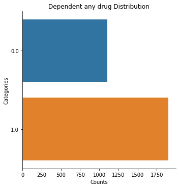
data.plot('target')

Dependent any drug: 3003 rows

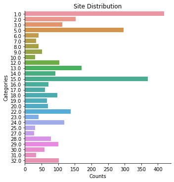
data.plot('Site')

Site: 3003 rows

data.plot_bivar('Site', 'Dependent any drug')

Site: 3003 rows
Dependent any drug: 3003 rows
Plotting 3003 overlap valid subjects.

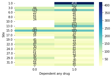
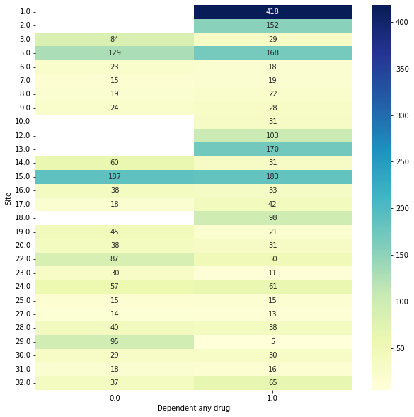
That bi-variate plot is a little hard to read… we can make it bigger though easy enough. Let’s say we also wanted to save it (we need to add show=False)

plt.figure(figsize=(10, 10))
data.plot_bivar('Site', 'Dependent any drug', show=False)
plt.savefig('site_by_drug.png', dpi=200)

Site: 3003 rows
Dependent any drug: 3003 rows
Plotting 3003 overlap valid subjects.

Okay next, we are going to define a custom validation strategy to use, which is essentially going to preserve subjects within the same train and test fold based on site.

Legacy Code

from BPt import CV
group_site = CV(groups='Site')

group_site = bp.CVStrategy(groups='Site')
group_site

CVStrategy(groups='Site')

We then can use this CV strategy as an argument when defining the train test split.

Legacy Code

ML.Train_Test_Split(test_size =.2, cv=group_site)

data = data.set_test_split(size=.2, cv_strategy=group_site, random_state=5)

Performing test split on: 3003 subjects.
random_state: 5
Test split size: 0.2

Performed train/test split
Train size: 2379
Test size:  624

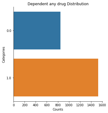
data.plot('target', subjects='train')
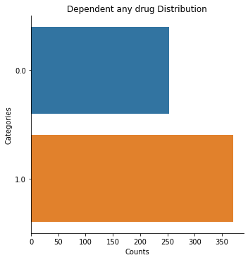
data.plot('target', subjects='test')

Dependent any drug: 2379 rows

Dependent any drug: 624 rows

Running ML

Next, we are going to evaluate some different machine learning models on the problem we have defined. Notably not much has changed here with respect to the old version, except some cosmetic changes like Problem_Spec to ProblemSpec. Also we have a new evaluate function instead of calling Evaluate via the ML object (ML.Evaluate).

# This just holds some commonly used values
ps = bp.ProblemSpec(subjects='train',
                    scorer=['matthews', 'roc_auc', 'balanced_accuracy'],
                    n_jobs=16)
ps

ProblemSpec(n_jobs=16, scorer=['matthews', 'roc_auc', 'balanced_accuracy'],
            subjects='train')

# Define a ModelPipeline to use with imputation, scaling and an elastic net
pipe = bp.ModelPipeline(imputers=[bp.Imputer(obj='mean', scope='float'),
                                  bp.Imputer(obj='median', scope='category')],
                        scalers=bp.Scaler('standard'),
                        model=bp.Model('elastic', params=1),
                        param_search=bp.ParamSearch(
                            search_type='DiscreteOnePlusOne', n_iter=64))
pipe.print_all()

ModelPipeline
-------------
imputers=\
[Imputer(obj='mean', scope='float'),
 Imputer(obj='median', scope='category')]

scalers=\
Scaler(obj='standard')

model=\
Model(obj='elastic', params=1)

param_search=\
ParamSearch(cv=CV(cv_strategy=CVStrategy()), n_iter=64,
            search_type='DiscreteOnePlusOne')

3-fold CV random splits

Let’s start by evaluating this model is a fairly naive way, just 3 folds of CV.

results = bp.evaluate(pipeline=pipe, dataset=data,
                      problem_spec=ps, cv=bp.CV(splits=3))
results

Predicting target = Dependent any drug
Using problem_type = binary
Using scope = all (defining a total of 163 features).
Evaluating 2379 total data points.

Train size: 1586 - Val size: 793
Fit fold in 15.781 seconds.
matthews: 0.45819711214039605
roc_auc: 0.8219843414397561
balanced_accuracy: 0.7347294394789718

Train size: 1586 - Val size: 793
Fit fold in 12.219 seconds.
matthews: 0.43270247791412836
roc_auc: 0.8060915258007118
balanced_accuracy: 0.7243174488434163

Train size: 1586 - Val size: 793
Fit fold in 11.532 seconds.
matthews: 0.4005078667838128
roc_auc: 0.7789128332642631
balanced_accuracy: 0.7066203895565686

BPtEvaluator
------------
mean_scores = {'matthews': 0.43046915227944577, 'roc_auc': 0.8023295668349103, 'balanced_accuracy': 0.721889092626319}
std_scores = {'matthews': 0.023604421407805696, 'roc_auc': 0.01778394323677345, 'balanced_accuracy': 0.0116032282095078}

Saved Attributes: ['estimators', 'preds', 'timing', 'train_subjects', 'val_subjects', 'feat_names', 'ps', 'mean_scores', 'std_scores', 'weighted_mean_scores', 'scores', 'fis_', 'coef_']

Available Methods: ['get_X_transform_df', 'get_preds_dfs', 'get_fis', 'get_coef_', 'permutation_importance']

Evaluated with:
ProblemSpec(n_jobs=16, problem_type='binary',
            scorer={'balanced_accuracy': make_scorer(balanced_accuracy_score),
                    'matthews': make_scorer(matthews_corrcoef),
                    'roc_auc': make_scorer(roc_auc_score, needs_threshold=True)},
            subjects='train', target='Dependent any drug')

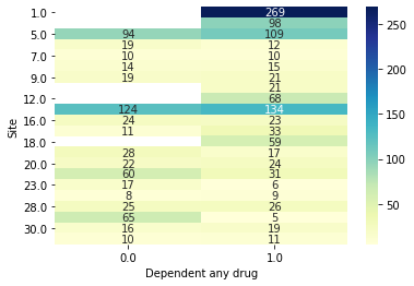
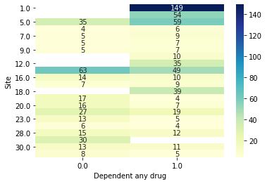
Notably this is likely going to give us overly optimistic results. Let’s look at just the Site’s drawn from the first evaluation fold to get a feel for why.

data.plot_bivar('Site', 'Dependent any drug', subjects=results.train_subjects[0])
data.plot_bivar('Site', 'Dependent any drug', subjects=results.val_subjects[0])

Site: 1586 rows
Dependent any drug: 1586 rows
Plotting 1586 overlap valid subjects.

Site: 793 rows
Dependent any drug: 793 rows
Plotting 793 overlap valid subjects.

Preserving Groups by Site

We can see that for example the 149 subjects from site 1 in the validation set had 269 subjects also from site 1 to potentially memorize site effects from! The confound is a site with only cases. One way we can account for this is through something we’ve already hinted at, using the group site cv from earlier. We can create a new CV object with this attribute.

site_cv = bp.CV(splits=3, cv_strategy=group_site)
site_cv

CV(cv_strategy=CVStrategy(groups='Site'))

results = bp.evaluate(pipeline=pipe, dataset=data,
                      problem_spec=ps, cv=site_cv)
results

BPtEvaluator
------------
mean_scores = {'matthews': 0.2806937010851929, 'roc_auc': 0.724342679133859, 'balanced_accuracy': 0.6448295419977427}
std_scores = {'matthews': 0.09542590294675868, 'roc_auc': 0.04969484135272, 'balanced_accuracy': 0.0595558011571011}

Saved Attributes: ['estimators', 'preds', 'timing', 'train_subjects', 'val_subjects', 'feat_names', 'ps', 'mean_scores', 'std_scores', 'weighted_mean_scores', 'scores', 'fis_', 'coef_']

Available Methods: ['get_preds_dfs', 'get_fis', 'get_coef_', 'permutation_importance']

Evaluated with:
ProblemSpec(n_jobs=16, problem_type='binary', scorer={'balanced_accuracy': make_scorer(balanced_accuracy_score), 'matthews': make_scorer(matthews_corrcoef), 'roc_auc': make_scorer(roc_auc_score, needs_threshold=True)}, subjects='train', target='Dependent any drug')

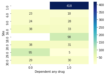
We can now make the same plots as before, confirming now that the sites are different.

data.plot_bivar('Site', 'Dependent any drug', subjects=results.train_subjects[0])
data.plot_bivar('Site', 'Dependent any drug', subjects=results.val_subjects[0])

Site: 1471 rows
Dependent any drug: 1471 rows
Plotting 1471 overlap valid subjects.

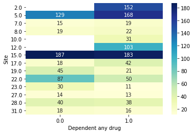
Site: 908 rows
Dependent any drug: 908 rows
Plotting 908 overlap valid subjects.

Another piece we might want to look at in this case is the weighted_mean_scores. That is, each of the splits has train and test sets of slightly different sizes, so how does the metric change if we weight it by the number of validation subjects in that fold

results.weighted_mean_scores

{'matthews': 0.2962912181056522,
 'roc_auc': 0.731185680809635,
 'balanced_accuracy': 0.6545156761514691}

results = bp.evaluate(pipeline=pipe, dataset=data,
                      problem_spec=ps, cv=3)
results

BPtEvaluator
------------
mean_scores = {'matthews': 0.4198523568381287, 'roc_auc': 0.8021293794313956, 'balanced_accuracy': 0.71695304741449}
std_scores = {'matthews': 0.05886752017766923, 'roc_auc': 0.020630146396151645, 'balanced_accuracy': 0.030556740029522838}

Saved Attributes: ['estimators', 'preds', 'timing', 'train_subjects', 'val_subjects', 'feat_names', 'ps', 'mean_scores', 'std_scores', 'weighted_mean_scores', 'scores', 'fis_', 'coef_']

Available Methods: ['get_preds_dfs', 'get_fis', 'get_coef_', 'permutation_importance']

Evaluated with:
ProblemSpec(n_jobs=16, problem_type='binary', scorer={'balanced_accuracy': make_scorer(balanced_accuracy_score), 'matthews': make_scorer(matthews_corrcoef), 'roc_auc': make_scorer(roc_auc_score, needs_threshold=True)}, subjects='train', target='Dependent any drug')

Other options?

What other options do we have to handle site with CV besides just the group splitting?

1. Explicit leave-out-site CV: Where every train set is composed of all sites but one, and the validation set is the left out site.

2. Use the train-only parameter in CV.

3. Only evaluate subjects from sites with both cases and controls.

Let’s try option 1 first.

Leave-out-site CV

# All we need to do for leave-out-site is specify that splits = Site
leave_out_site_cv = bp.CV(splits='Site')

# This will actually raise an error
try:
    results = bp.evaluate(pipeline=pipe, dataset=data,
                          problem_spec=ps, cv=leave_out_site_cv)
except Exception as exc:
    print(exc)

Only one class present in y_true. ROC AUC score is not defined in that case.

/home/sage/anaconda3/envs/bpt/lib/python3.9/site-packages/sklearn/metrics/_classification.py:870: RuntimeWarning: invalid value encountered in double_scalars
  mcc = cov_ytyp / np.sqrt(cov_ytyt * cov_ypyp)

Uh oh looks like this option actually failed. What happened? Well basically since we have sites with only one class, we are trying to compute metrics that require two classes. Let’s try again this time just using scorers that can work in the case of only one class.

results = bp.evaluate(pipeline=pipe, dataset=data, scorer='accuracy',
                      problem_spec=ps, cv=leave_out_site_cv)

results.mean_scores, results.std_scores, results.weighted_mean_scores

({'accuracy': 0.6236689337343281},
 {'accuracy': 0.19902767857831596},
 {'accuracy': 0.6658259773013872})

The problem here is accuracy is likely a pretty bad metric, especially for the sites which have both cases and controls, but a skewed distribution. In general using the group preserving by Site is likely a better option.

Train-only subjects

One optional way of handling these subjects from sites with only cases or only controls is to just never evaluate them. To instead always treat them as train subjects. We can notably then either use random splits or group preserving by CV.

def check_imbalanced(df):
    as_int = df['Dependent any drug'].astype('int')
    return np.sum(as_int) == len(as_int)

# Apply function to check if each site has all the same target variable
is_imbalanced = data.groupby('Site').apply(check_imbalanced)

# Note these are internal values, not the original ones
imbalanced_sites = np.flatnonzero(is_imbalanced)

# We can specify just these subjects using the ValueSubset wrapper
imbalanced_subjs = bp.ValueSubset('Site', values=imbalanced_sites, decode_values=False)

# Now define our new version of the group site cv
site_cv_tr_only = bp.CV(splits=3, cv_strategy=group_site,
                        train_only_subjects=imbalanced_subjs)

# And evaluate
results = bp.evaluate(pipeline=pipe, dataset=data,
                      problem_spec=ps, cv=site_cv_tr_only)
results

BPtEvaluator
------------
mean_scores = {'matthews': 0.024294039432900597, 'roc_auc': 0.5292721521624003, 'balanced_accuracy': 0.5116503104881627}
std_scores = {'matthews': 0.0818023189639453, 'roc_auc': 0.053461117751205205, 'balanced_accuracy': 0.04147838671486171}

Saved Attributes: ['estimators', 'preds', 'timing', 'train_subjects', 'val_subjects', 'feat_names', 'ps', 'mean_scores', 'std_scores', 'weighted_mean_scores', 'scores', 'fis_', 'coef_']

Available Methods: ['get_preds_dfs', 'get_fis', 'get_coef_', 'permutation_importance']

Evaluated with:
ProblemSpec(n_jobs=16, problem_type='binary', scorer={'balanced_accuracy': make_scorer(balanced_accuracy_score), 'matthews': make_scorer(matthews_corrcoef), 'roc_auc': make_scorer(roc_auc_score, needs_threshold=True)}, subjects='train', target='Dependent any drug')

The take-away here is maybe a little bleak. Essentially it is saying that some of the high scores we got earlier might have been in large part due to scores from the imbalanced sites.

# And we can also run a version with just random splits
tr_only_cv = bp.CV(splits=3, train_only_subjects=imbalanced_subjs)

# And evaluate
results = bp.evaluate(pipeline=pipe, dataset=data,
                      problem_spec=ps, cv=tr_only_cv)
results

BPtEvaluator
------------
mean_scores = {'matthews': 0.23754373855512448, 'roc_auc': 0.6581411778771414, 'balanced_accuracy': 0.6117532215243421}
std_scores = {'matthews': 0.028251718001276915, 'roc_auc': 0.00840487420017697, 'balanced_accuracy': 0.01031391488070083}

Saved Attributes: ['estimators', 'preds', 'timing', 'train_subjects', 'val_subjects', 'feat_names', 'ps', 'mean_scores', 'std_scores', 'weighted_mean_scores', 'scores', 'fis_', 'coef_']

Available Methods: ['get_preds_dfs', 'get_fis', 'get_coef_', 'permutation_importance']

Evaluated with:
ProblemSpec(n_jobs=16, problem_type='binary', scorer={'balanced_accuracy': make_scorer(balanced_accuracy_score), 'matthews': make_scorer(matthews_corrcoef), 'roc_auc': make_scorer(roc_auc_score, needs_threshold=True)}, subjects='train', target='Dependent any drug')

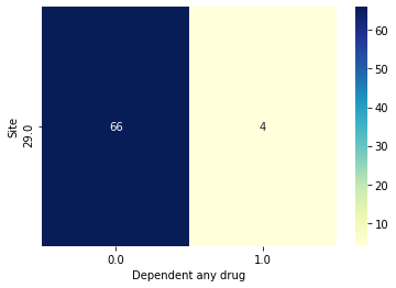
While this version with random splits does better, we are still notably ignoring the distribution of case to control in the sites with both cases and controls. Based on the group preserving results what it seems like is going on is that when subjects from the same site are split across validation folds, the classifier might be able to just memorize Site instead of the effect of interest. Lets use Site 29 as an example.

Let’s look at just fold 1 first.

# The train and val subjects from fold 0
tr_subjs = results.train_subjects[0]
val_subjs = results.val_subjects[0]

# An object specifying just site 29's subjects
site29 = bp.ValueSubset('Site', 29, decode_values=True)

# Get the intersection w/ intersection obj
site_29_tr = bp.Intersection([tr_subjs, site29])
site_29_val = bp.Intersection([val_subjs, site29])

# Plot
data.plot_bivar('Site', 'Dependent any drug', subjects=bp.Intersection([tr_subjs, site29]))
data.plot_bivar('Site', 'Dependent any drug', subjects=bp.Intersection([val_subjs, site29]))

# Grab just the subjects as actual index
val_subjs = data.get_subjects(site_29_val)

# Get a dataframe with the predictions made for just fold0
preds_df_fold0 = results.get_preds_dfs()[0]

# Let's see predictions for just these validation subjects
preds_df_fold0.loc[val_subjs]

Site: 70 rows
Dependent any drug: 70 rows
Plotting 70 overlap valid subjects.

Site: 30 rows
Dependent any drug: 30 rows
Plotting 30 overlap valid subjects.

	predict	predict_proba	decision_function	y_true
3458	0.0	0.810241	-1.451580	0.0
3459	0.0	0.902262	-2.222618	0.0
3462	0.0	0.976899	-3.744522	0.0
3470	0.0	0.954009	-3.032217	0.0
3478	0.0	0.964846	-3.312243	0.0
3479	0.0	0.900526	-2.203087	0.0
3482	0.0	0.946305	-2.869253	0.0
3484	0.0	0.681535	-0.760837	0.0
3485	0.0	0.924836	-2.509949	0.0
3486	0.0	0.957875	-3.124076	0.0
3494	0.0	0.870815	-1.908185	0.0
3497	0.0	0.959444	-3.163663	0.0
3498	0.0	0.877308	-1.967185	0.0
3502	0.0	0.892309	-2.114550	0.0
3503	0.0	0.946427	-2.871650	1.0
3507	0.0	0.968260	-3.417921	0.0
3509	0.0	0.961510	-3.218103	0.0
3512	0.0	0.907378	-2.282028	0.0
3517	0.0	0.976704	-3.735907	0.0
3521	0.0	0.665222	-0.686655	0.0
3523	0.0	0.699328	-0.844100	0.0
3423	0.0	0.951770	-2.982337	0.0
3429	0.0	0.603810	-0.421364	0.0
3434	0.0	0.955454	-3.065661	0.0
3437	0.0	0.934065	-2.650873	0.0
3442	0.0	0.912519	-2.344782	0.0
3443	0.0	0.927844	-2.554032	0.0
3447	0.0	0.916637	-2.397506	0.0
3453	0.0	0.945561	-2.854691	0.0
3455	0.0	0.745451	-1.074496	0.0

We can see that it has learned to just predict 0 for every subject, which because of the imbalance is right most of the time, but really doesn’t tell us if it has learned to predict site or substance dependence.

Drop imbalanced subjects

The last option was just don’t use the imbalanced subjects at all. We will do this by indexing only the balanced sites

# Note the ~ before the previously defined is_imbalanced
balanced_sites = np.flatnonzero(~is_imbalanced)

# We can specify just these subjects using the ValueSubset wrapper
balanced_subjs = bp.ValueSubset('Site', values=balanced_sites, decode_values=False)

# Evaluate with site preserving cv from earlier but now using just the balanced train subjects
train_just_balanced = bp.Intersection(['train', balanced_subjs])

results = bp.evaluate(pipeline=pipe, dataset=data,
                      subjects=train_just_balanced,
                      problem_spec=ps, cv=site_cv)
results

BPtEvaluator
------------
mean_scores = {'matthews': 0.23079311975258734, 'roc_auc': 0.6494071534373412, 'balanced_accuracy': 0.6141868842892168}
std_scores = {'matthews': 0.09467372271946288, 'roc_auc': 0.07189605086562514, 'balanced_accuracy': 0.05165558889230518}

Saved Attributes: ['estimators', 'preds', 'timing', 'train_subjects', 'val_subjects', 'feat_names', 'ps', 'mean_scores', 'std_scores', 'weighted_mean_scores', 'scores', 'fis_', 'coef_']

Available Methods: ['get_preds_dfs', 'get_fis', 'get_coef_', 'permutation_importance']

Evaluated with:
ProblemSpec(n_jobs=16, problem_type='binary', scorer={'balanced_accuracy': make_scorer(balanced_accuracy_score), 'matthews': make_scorer(matthews_corrcoef), 'roc_auc': make_scorer(roc_auc_score, needs_threshold=True)}, subjects=Intersection(['train', ValueSubset(name=Site, values=[ 2  3  4  5  6  7 11 12 13 14 16 17 18 19 20 21 22 23 24 25 26 27], decode_values=False)]), target='Dependent any drug')

This actually seems to show that the imbalanced site confound with doesn’t just corrupt cross validated results, but also actively impedes the model learning the real relationship. That we are better off just not using subjects with from sites with only cases. Yikes.

Likewise, we can do the random split strategy again too.

results = bp.evaluate(pipeline=pipe, dataset=data,
                      subjects=train_just_balanced,
                      problem_spec=ps, cv=bp.CV(splits=3))
results

BPtEvaluator
------------
mean_scores = {'matthews': 0.3099741843096915, 'roc_auc': 0.7185050035507189, 'balanced_accuracy': 0.6557306499974717}
std_scores = {'matthews': 0.05501720339208484, 'roc_auc': 0.030948171887409684, 'balanced_accuracy': 0.02748782703232899}

Saved Attributes: ['estimators', 'preds', 'timing', 'train_subjects', 'val_subjects', 'feat_names', 'ps', 'mean_scores', 'std_scores', 'weighted_mean_scores', 'scores', 'fis_', 'coef_']

Available Methods: ['get_preds_dfs', 'get_fis', 'get_coef_', 'permutation_importance']

Evaluated with:
ProblemSpec(n_jobs=16, problem_type='binary', scorer={'balanced_accuracy': make_scorer(balanced_accuracy_score), 'matthews': make_scorer(matthews_corrcoef), 'roc_auc': make_scorer(roc_auc_score, needs_threshold=True)}, subjects=Intersection(['train', ValueSubset(name=Site, values=[ 2  3  4  5  6  7 11 12 13 14 16 17 18 19 20 21 22 23 24 25 26 27], decode_values=False)]), target='Dependent any drug')

Also, we could run it with a leave-out-site CV. Now we can use the normal metrics.

results = bp.evaluate(pipeline=pipe, dataset=data,
                      subjects=train_just_balanced,
                      problem_spec=ps, cv=leave_out_site_cv)
results

/home/sage/anaconda3/envs/bpt/lib/python3.9/site-packages/sklearn/metrics/_classification.py:870: RuntimeWarning: invalid value encountered in double_scalars
  mcc = cov_ytyp / np.sqrt(cov_ytyt * cov_ypyp)

BPtEvaluator
------------
mean_scores = {'matthews': 0.14755625865911742, 'roc_auc': 0.6060559623948263, 'balanced_accuracy': 0.5636346829506975}
std_scores = {'matthews': 0.17026794856315272, 'roc_auc': 0.12014100381868857, 'balanced_accuracy': 0.076467544201846}

Saved Attributes: ['estimators', 'preds', 'timing', 'train_subjects', 'val_subjects', 'feat_names', 'ps', 'mean_scores', 'std_scores', 'weighted_mean_scores', 'scores', 'fis_', 'coef_']

Available Methods: ['get_preds_dfs', 'get_fis', 'get_coef_', 'permutation_importance']

Evaluated with:
ProblemSpec(n_jobs=16, problem_type='binary', scorer={'balanced_accuracy': make_scorer(balanced_accuracy_score), 'matthews': make_scorer(matthews_corrcoef), 'roc_auc': make_scorer(roc_auc_score, needs_threshold=True)}, subjects=Intersection(['train', ValueSubset(name=Site, values=[ 2  3  4  5  6  7 11 12 13 14 16 17 18 19 20 21 22 23 24 25 26 27], decode_values=False)]), target='Dependent any drug')

Results Summary

To summarize, of all of the above different iterations. Only the results from the versions where subjects from case-only sites are treated as train-only or dropped and evaluated group-preserving by site are likely un-biased! The leave-out-site CV results should be okay too, but let’s skip those for now.

Train Only Scores: mean_scores = {‘matthews’: 0.024294039432900597, ‘roc_auc’: 0.5292721521624003, ‘balanced_accuracy’: 0.5116503104881627}

Dropped Scores: mean_scores = {‘matthews’: 0.23079311975258734, ‘roc_auc’: 0.6494071534373412, ‘balanced_accuracy’: 0.6141868842892168}

By these interm results we can with some confidence conclude dropping subjects is the way to go, unless we want to dig deeper…

Disentangle Target and Site?

Can information on dependance from case-only sites be some how disentangled from site?

This actually leads to a follow up a question. Namely is there any way to extract usable information from case-only site subjects? This question I actually investigated more deeply in https://onlinelibrary.wiley.com/doi/full/10.1002/hbm.25248 The idea of train-only subjects is actually from this paper, though it still has some important differences then the way we formulated it.

The key piece in the paper which we haven’t tried to do yet is centered around the problem of the classifier learning site related information instead of dependence related information in the train-only setup. We essentially need a way of forcing the classifier to learn this. The way proposed in the paper proposes that maybe we can by restricting the features provided to the classifier, give it only features related to dependence and not those related to site. In order to do this, we need to add a feature selection step.

There are different ways to compose the problem, but we will specify the feature selection step as a seperate layer of nesting, importantly one that is evaluated according to the same site_cv_tr_only that we will be evaluating with. Remember the goal here is to select features which help us learn to predict useful information from case only sites, i.e., with feature only related to Dependence and not site!

# Same imputer and scaler
imputers = [bp.Imputer(obj='mean', scope='float'),
            bp.Imputer(obj='median', scope='category')]
scaler = bp.Scaler('standard')

# This object will be used to set features as an array of binary hyper-parameters
feat_selector = bp.FeatSelector('selector', params=1)

# This param search is responsible for optimizing the selected features from feat_selector
param_search = bp.ParamSearch('RandomSearch',
                              n_iter=16,
                              cv=site_cv_tr_only)

# We create a nested elastic net model to optimize - no particular CV should be okay
random_search = bp.ParamSearch('RandomSearch', n_iter=16)
elastic_search = bp.Model('elastic', params=1,
                          param_search=random_search)

# Put it all together in a pipeline
fs_pipe = bp.Pipeline(imputers + [scaler, feat_selector, elastic_search],
                      param_search=param_search)

Note: This may take a while to evaluate as we now have two levels of parameters to optimize, e.g., for each choice of features, we need to train a nested elastic net.

results = bp.evaluate(pipeline=fs_pipe, dataset=data,
                      problem_spec=ps, cv=site_cv_tr_only)
results

BPtEvaluator
------------
mean_scores = {'matthews': 0.02346740168044174, 'roc_auc': 0.4992373334460878, 'balanced_accuracy': 0.511308005873143}
std_scores = {'matthews': 0.09763704971436771, 'roc_auc': 0.06654364664577839, 'balanced_accuracy': 0.04908589456453536}

Saved Attributes: ['estimators', 'preds', 'timing', 'train_subjects', 'val_subjects', 'feat_names', 'ps', 'mean_scores', 'std_scores', 'weighted_mean_scores', 'scores']

Available Methods: ['get_preds_dfs', 'permutation_importance']

Evaluated with:
ProblemSpec(n_jobs=16, problem_type='binary', scorer={'balanced_accuracy': make_scorer(balanced_accuracy_score), 'matthews': make_scorer(matthews_corrcoef), 'roc_auc': make_scorer(roc_auc_score, needs_threshold=True)}, subjects='train', target='Dependent any drug')

Unfortunetly this doesn’t seem to work. Notably we still arn’t quite following the method from the paper, which performs a meta-analysis on the results from the feature search to find overlapping subsets of features. As of the time of writing this example, a simmilar strategy has not been able to be easily integrated into BPt.

The above method still has a few problems, one being severe overfitting. Namely, because a number of subjects are reserved in train-only roles, the same small number of subjects are being used over and over in cross-validation.

We can confirm this intutiton by comparing the best score achieved internally for each set of features w/ how they score in the outer cross validation.

-results.estimators[0].best_score_, results.scores['matthews'][0]

(0.034082343012732844, 0.1394079745869329)

-results.estimators[1].best_score_, results.scores['matthews'][1]

(0.15037612204051184, -0.09944769119313912)

-results.estimators[2].best_score_, results.scores['matthews'][2]

(0.10307484584144071, 0.030441921647531428)

These values are quite different to say the least. Part of the problem again is that such a small amount of data is being used to determine generalization. What if instead of a the 3-fold group preserving train only feature selection CV, we instead used a leave-out-site scheme on site with train only? I doubt it will help, but let’s see…

leave_out_site_tr_only_cv = bp.CV(splits='Site',
                                  train_only_subjects=imbalanced_subjs)

fs_pipe.param_search = bp.ParamSearch(
    'RandomSearch', n_iter=16,
    cv=leave_out_site_tr_only_cv)

results = bp.evaluate(pipeline=fs_pipe, dataset=data,
                      problem_spec=ps, cv=site_cv_tr_only)
results

BPtEvaluator
------------
mean_scores = {'matthews': 0.03667173630581328, 'roc_auc': 0.5248868808677055, 'balanced_accuracy': 0.5178404766273731}
std_scores = {'matthews': 0.11389312167894736, 'roc_auc': 0.06057589628452694, 'balanced_accuracy': 0.05676567744096608}

Saved Attributes: ['estimators', 'preds', 'timing', 'train_subjects', 'val_subjects', 'feat_names', 'ps', 'mean_scores', 'std_scores', 'weighted_mean_scores', 'scores']

Available Methods: ['get_preds_dfs', 'permutation_importance']

Evaluated with:
ProblemSpec(n_jobs=16, problem_type='binary', scorer={'balanced_accuracy': make_scorer(balanced_accuracy_score), 'matthews': make_scorer(matthews_corrcoef), 'roc_auc': make_scorer(roc_auc_score, needs_threshold=True)}, subjects='train', target='Dependent any drug')

This does a little better. But only slightly. What if we also used this leave-out site strategy for the outer loop? This would be to address the issue that the outer CV has the same problem as the inner, where the validation set is overly specific and small in some folds.

results = bp.evaluate(pipeline=fs_pipe,
                      dataset=data,
                      problem_spec=ps,
                      cv=leave_out_site_tr_only_cv,
                      eval_verbose=1)
results

Predicting target = Dependent any drug
Using problem_type = binary
Using scope = all defining an initial total of 163 features.
Evaluating 2379 total data points.

Train shape = (2082, 163) (number of data points x number of feature)
Val shape = (297, 163) (number of data points x number of feature)
Fit fold in 433.108 seconds.
matthews: 0.27971196025033845
roc_auc: 0.6950904392764857
balanced_accuracy: 0.6410575858250277
Train shape = (2338, 163) (number of data points x number of feature)
Val shape = (41, 163) (number of data points x number of feature)
Fit fold in 488.837 seconds.
matthews: 0.0
roc_auc: 0.4492753623188406
balanced_accuracy: 0.5
Train shape = (2345, 163) (number of data points x number of feature)
Val shape = (34, 163) (number of data points x number of feature)

/home/sage/anaconda3/envs/bpt/lib/python3.9/site-packages/sklearn/metrics/_classification.py:870: RuntimeWarning: invalid value encountered in double_scalars
  mcc = cov_ytyp / np.sqrt(cov_ytyt * cov_ypyp)

Fit fold in 448.277 seconds.
matthews: -0.1604088343952626
roc_auc: 0.46315789473684216
balanced_accuracy: 0.42280701754385963
Train shape = (2338, 163) (number of data points x number of feature)
Val shape = (41, 163) (number of data points x number of feature)
Fit fold in 470.407 seconds.
matthews: -0.019138755980861243
roc_auc: 0.47368421052631576
balanced_accuracy: 0.49043062200956933
Train shape = (2327, 163) (number of data points x number of feature)
Val shape = (52, 163) (number of data points x number of feature)
Fit fold in 448.843 seconds.
matthews: 0.3354656500760583
roc_auc: 0.6979166666666666
balanced_accuracy: 0.6636904761904762
Train shape = (2009, 163) (number of data points x number of feature)
Val shape = (370, 163) (number of data points x number of feature)
Fit fold in 437.145 seconds.
matthews: 0.020177568979434148
roc_auc: 0.49300137342567435
balanced_accuracy: 0.5099646415943426
Train shape = (2308, 163) (number of data points x number of feature)
Val shape = (71, 163) (number of data points x number of feature)
Fit fold in 451.353 seconds.
matthews: 0.0
roc_auc: 0.5223285486443381
balanced_accuracy: 0.5
Train shape = (2319, 163) (number of data points x number of feature)
Val shape = (60, 163) (number of data points x number of feature)

/home/sage/anaconda3/envs/bpt/lib/python3.9/site-packages/sklearn/metrics/_classification.py:870: RuntimeWarning: invalid value encountered in double_scalars
  mcc = cov_ytyp / np.sqrt(cov_ytyt * cov_ypyp)

Fit fold in 454.574 seconds.
matthews: -0.12598815766974242
roc_auc: 0.5039682539682541
balanced_accuracy: 0.44047619047619047
Train shape = (2313, 163) (number of data points x number of feature)
Val shape = (66, 163) (number of data points x number of feature)
Fit fold in 458.078 seconds.
matthews: 0.053121271525973054
roc_auc: 0.5089947089947089
balanced_accuracy: 0.5253968253968253
Train shape = (2310, 163) (number of data points x number of feature)
Val shape = (69, 163) (number of data points x number of feature)
Fit fold in 452.421 seconds.
matthews: 0.2622746101092192
roc_auc: 0.6256366723259762
balanced_accuracy: 0.6294567062818336
Train shape = (2242, 163) (number of data points x number of feature)
Val shape = (137, 163) (number of data points x number of feature)
Fit fold in 442.038 seconds.
matthews: -0.11597093720775255
roc_auc: 0.5342528735632184
balanced_accuracy: 0.4574712643678161
Train shape = (2338, 163) (number of data points x number of feature)
Val shape = (41, 163) (number of data points x number of feature)
Fit fold in 456.392 seconds.
matthews: 0.2313602894352951
roc_auc: 0.6515151515151514
balanced_accuracy: 0.6257575757575757
Train shape = (2352, 163) (number of data points x number of feature)
Val shape = (27, 163) (number of data points x number of feature)
Fit fold in 462.279 seconds.
matthews: -0.12507270025494252
roc_auc: 0.37912087912087916
balanced_accuracy: 0.43956043956043955
Train shape = (2301, 163) (number of data points x number of feature)
Val shape = (78, 163) (number of data points x number of feature)
Fit fold in 453.980 seconds.
matthews: 0.12403989506994083
roc_auc: 0.5671052631578948
balanced_accuracy: 0.5565789473684211
Train shape = (2279, 163) (number of data points x number of feature)
Val shape = (100, 163) (number of data points x number of feature)
Fit fold in 442.766 seconds.
matthews: 0.06294058066909786
roc_auc: 0.4231578947368421
balanced_accuracy: 0.5368421052631579
Train shape = (2320, 163) (number of data points x number of feature)
Val shape = (59, 163) (number of data points x number of feature)
Fit fold in 450.422 seconds.
matthews: -0.005703586973049607
roc_auc: 0.48160919540229885
balanced_accuracy: 0.4982758620689655
Train shape = (2345, 163) (number of data points x number of feature)
Val shape = (34, 163) (number of data points x number of feature)
Fit fold in 460.327 seconds.
matthews: 0.10213764617139019
roc_auc: 0.6423611111111112
balanced_accuracy: 0.5451388888888888

BPtEvaluator
------------
mean_scores = {'matthews': 0.05405567645912566, 'roc_auc': 0.5360103823230292, 'balanced_accuracy': 0.5284061852113758}
std_scores = {'matthews': 0.14703361948297453, 'roc_auc': 0.0926704447511229, 'balanced_accuracy': 0.07192589246275141}

Saved Attributes: ['estimators', 'preds', 'timing', 'train_subjects', 'val_subjects', 'feat_names', 'ps', 'mean_scores', 'std_scores', 'weighted_mean_scores', 'scores']

Available Methods: ['get_preds_dfs', 'permutation_importance']

Evaluated with:
ProblemSpec(n_jobs=16, problem_type='binary', scorer={'balanced_accuracy': make_scorer(balanced_accuracy_score), 'matthews': make_scorer(matthews_corrcoef), 'roc_auc': make_scorer(roc_auc_score, needs_threshold=True)}, subjects='train', target='Dependent any drug')

Seeing the results for each site seperately with the verbose option really makes some of the problem clear, namely that a number of small sites don’t seem to generalize well. This is simmilar to what we saw in the case of using leave-out-site with case-only subjects dropped, where we had a huge std in roc auc between folds.

Another potential problem with doing leave-out-site is that the way the underlying data was collected, different sites will have subjects with dependence to different substances. This can certainly cause issues, as say our classifier only learns to classify alcohol dependence (the strongest signal), then it will do poorly on sites for other substances. Which is good in one way, that it lets us know the classifier is not generalizing, but it doesn’t solve the generalization problem.

Anyways, that will end this example for now. Leaving the problem of how to best exploit information from case-only sites as an open question (though if interested, a more faithful reproduction of the method presented in https://onlinelibrary.wiley.com/doi/full/10.1002/hbm.25248 might prove to be fruitful. Specifically, in the end only using a few, maybe 3-4, features, which is notably quite different then what we are trying above, i.e., trying just 16 random sets of features).